Pareto charts are popular quality control tools that make it easy for you to identify the most important issues. They are a combination of bar and line charts with the longest bars (major issues) on the left. In Microsoft Excel, you can create and customize a Pareto chart.
The benefit of a Pareto chart
The main benefit of a Pareto chart structure is that you can quickly spot what you need to focus on the most.. Starting from the left side, the bars go from highest to lowest. The line at the top shows a cumulative total percentage.
You regularly have data categories with representative numbers. Then, can analyze data in relation to frequency of occurrences. In general, those frequencies are focused on cost, the amount or the time.
RELATED: How to save time with Excel themes
Create a Pareto chart in Excel
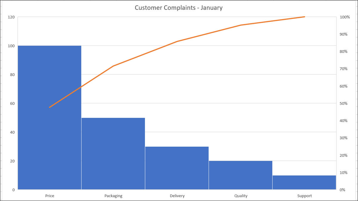
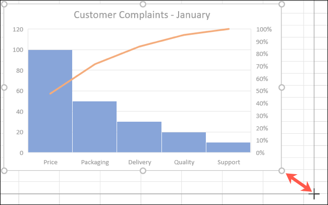
For this tutorial, we will use data for customer complaints. We have five categories for our clients' complaints and numbers for the number of complaints received for each category.
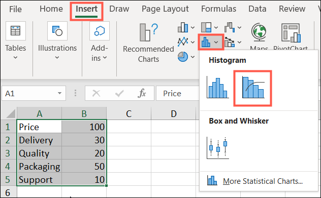
Get started by selecting the data for your chart. The order in which your data resides in the cells is not essential because the Pareto chart structures it automatically.
Go to the Insert tab and click the drop-down arrow “Insert stat chart”. Please select “Pareto” in the Histogram section of the menu. Remember, a Pareto chart is an ordered histogram chart.
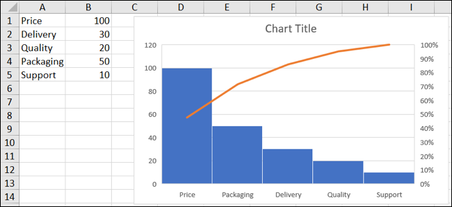
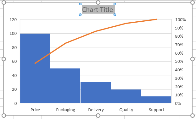
And so, a Pareto chart appears on your spreadsheet. You will see your categories as the horizontal axis and your numbers as the vertical axis. On the right side of the graph are the percentages as the vertical secondary axis.
Now we can clearly see from this Pareto chart that we need to have some discussion about Price because that is our biggest complaint from customers.. And we can focus less on support because we don't get as many complaints in that category..
Customize a Pareto chart
If you plan to share your chart with other people, you may want to fix it a bit or add and remove items from the chart.
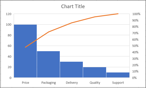
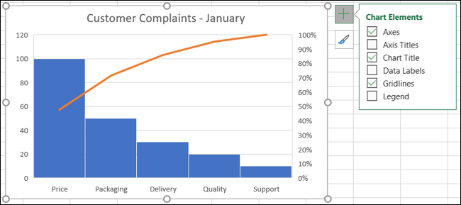
You can start by changing the title of the default chart. Click in the text box and add the title you want to use.
In Windows, you will see helpful tools on the right when you select the chart. The first is for the items in the chart, so you can snap the grid lines, data labels and legend. The second is for Chart Styles, allowing you to choose a theme for the graphic or a color scheme.
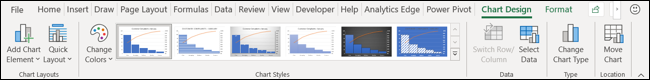
You can also choose the graphic and go to the Graphic Design tab that is displayed. The ribbon provides you with tools to change the design or style, add or remove items from the chart or adjust your data selection.
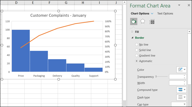
One more way to customize your Pareto chart is by double clicking to open the Format chart area sidebar. Has tabs for Fill and line, Effects and Size and properties. Because, can add a border, a shadow or a specific height and width.
You can also move your Pareto chart by dragging it or resize it by dragging it in or out from a corner or edge..
For more types of charts, take a look at how to create geomap chart or make bar chart in Excel.