How to combine or group pie charts in Microsoft Excel

Pie charts are popular in Excel, but they are limited. You will have to choose for yourself between using multiple pie charts or forgoing some flexibility in favor of readability by combining them. If you want to combine them, here we show you how.

As an example, the following pie chart shows people's responses to a question.

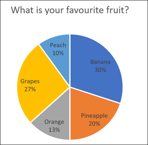
This is good, but it can be tricky if you have multiple pie charts.

Pie charts can only display a series of values. Then, if you have multiple series and want to present data with pie charts, need several pie charts.

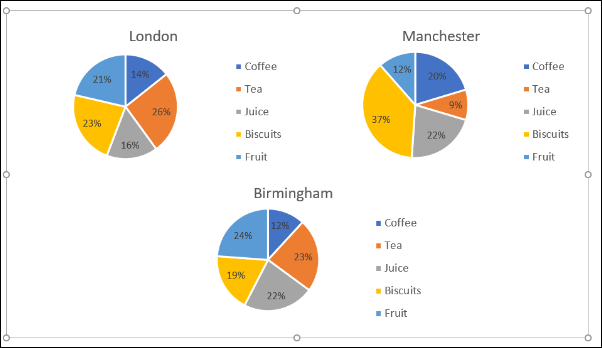
The next image shows the contribution to total revenue of five products in three different cities. We have a pie chart for each city with the data ranges shown above.

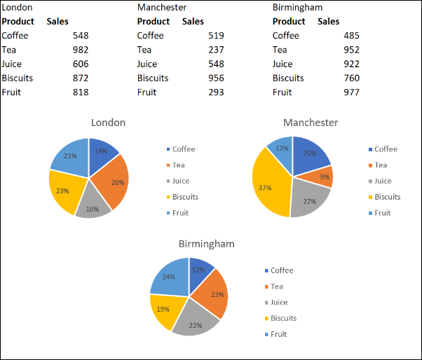
This enables us to compare product sales in different cities. But there are complications when we want to change them all consistently or see them as a single figure..

In this post, we will look at three different approaches to combine pie charts.

Consolidate data from multiple charts

The first approach seeks to combine the data used by the pie charts.

It makes sense to display one pie chart instead of three. This would create more space in the report and mean less “eye tennis” by the reader.

Despite this, in this example, will come at the cost of city comparison.

The easiest and fastest way to combine the data from the three pie charts is to use the Consolidate tool in Excel.

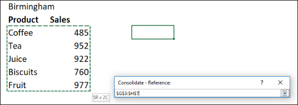
Let's consolidate the data shown below.

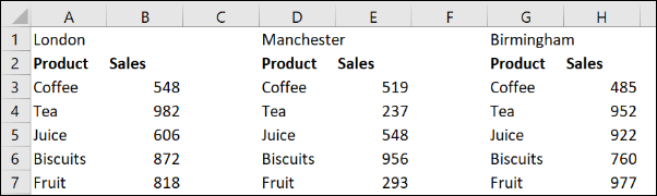
Click a cell on the sheet where the consolidated data will be placed. Click Data> Consolidate on the tape.

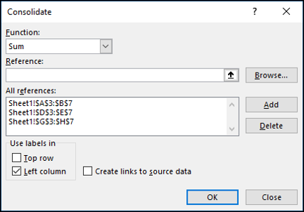
The Consolidate window opens.

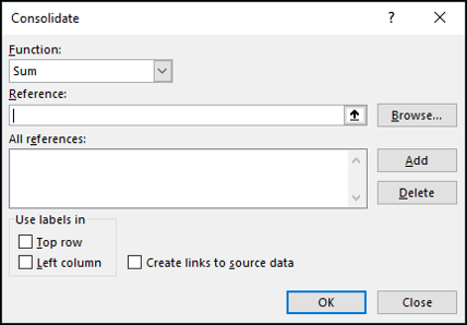
We will use the Sum function to total the sales of the three cities.

Next, we have to collect all the references that we want to consolidate. Click on the box “Reference”, select the first range, and then click “Add”.

Repeat this step for the other references.

Check the box “Left column” since the product name is to the left of the values in our data. Click OK.”

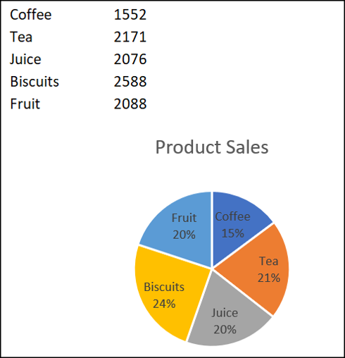
We now have a consolidated range from which to create our pie chart.

This pie chart makes it easy to see the contribution of each type of product to total revenue., but we lose the comparison between each city that we had with three different graphs.

Combine pie chart into one shape

Another reason you may want to combine pie charts is so that you can move and resize them as one..

Click on the first chart and then hold down the Ctrl key while clicking each of the other charts to select them all.

Click Format> Group> Group.

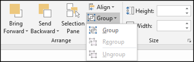
All pie charts are now combined into a single figure. They will move and resize as a single image.

Choose different charts to see your data

Even though this post is about combining pie charts, another alternative would be to opt for a different type of graph. Pie charts aren't the only way to visualize parts of a whole.

A good alternative would be the stacked column chart.

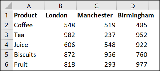
Take the example data below. These are the data used in this post, but now combined in a table.

Select the cell range and click Insert> Column chart.

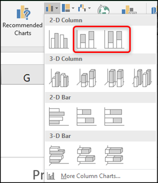
There are two types of stacked columns to select. The first will present your data as shown below.

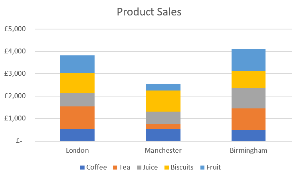
It's like having three pie charts on one chart.

Does an excellent job of showing the contribution of values ​​in each city, at the same time that it allows us to compare costs between cities.

As an example, we can see that Manchester produced the lowest income and that the tea and fruit sales were low compared to the other stores.

The second stacked column chart option would present your data as shown below.

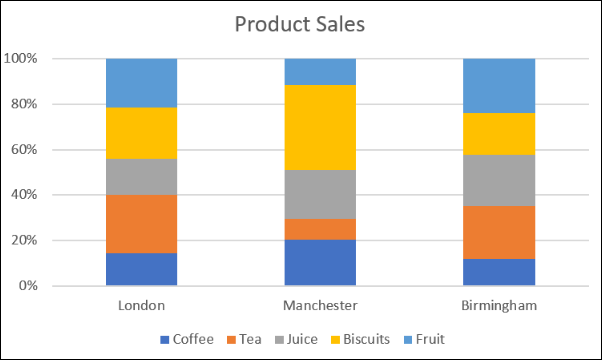
This uses a percentage on the axis.

Therefore we lose the ability to see that Manchester produced the lowest income, but it can give us a better focus on the relative contribution. As an example, most of the Manchester store's sales were cookies.

You can click the button “Change row / column” on the Design tab to switch the data between the axis and the legend.

Depending on your motives, there are different alternatives to combine pie charts into a single figure. This post explored three techniques as solutions to three different presentation scenarios..