
Your Excel data changes often, so it's useful to create a dynamic defined range that automatically expands and contracts to the size of your data range. Lets see how.
When using a defined dynamic range, you won't need to manually edit the ranges of your formulas, pivot charts and tables when data changes. This will happen automatically.
Two formulas are used to create dynamic ranges: OFFSET e INDEX. This post will focus on the use of the INDEX function, since it is a more efficient approach. OFFSET is a volatile function and can slow down large spreadsheets.
Create a defined dynamic range in Excel
For our first example, we have the single column data list seen below.
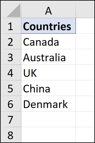
We need this to be dynamic so if more countries are added or removed, the range updates automatically.
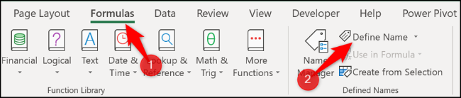
For this example, we want to avoid header cell. As such, we want the range $ A $ 2: $ A $ 6, but dynamic. Do this by clicking on Formulas> Set Name.
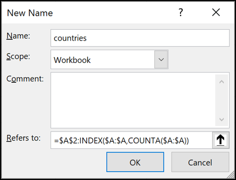
Scribe “countries” in the frame “Name” and then enter the formula below in the box “Refers to”.
=$A$2:INDEX($A:$A,COUNTA($A:$A))
Typing this equation into a cell on your spreadsheet and then copying it into the New name box is sometimes faster and easier.
How does this work?
The first part of the formula specifies the starting cell of the range (A2 in our case) and then follow the range operator (:).
=$A$2:
Using the range operator forces the INDEX function to return a range instead of the value of a cell. The INDEX function is then used with the COUNT function. COUNT counts the number of cells that are not blank in column A (six in our case).
INDEX($A:$A,COUNTA($A:$A))
This formula asks the INDEX function to return the range of the last non-blank cell in column A ($ A $ 6).
The end result is $ A $ 2: $ A $ 6, and due to the COUNT function, it is dynamic, since it will find the last row. You can now use this name defined by “countries” within a data validation rule, formula, graphic or where we need to refer to the names of all the countries.
Create a defined bi-directional dynamic range
The first example was only dynamic in height. Despite this, with a slight modification and another function COUNT, you can create a range that is dynamic in both height and width.
In this example, we will use the data shown below.
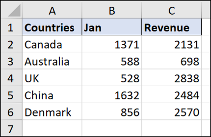
This time, we will create a defined dynamic range, which includes the headers. Click Formulas> Set Name.
Scribe “sales” in the frame “Name” and enter the formula below in the box “Refers to”.
=$A$1:INDEX($1:$1048576,COUNTA($A:$A),COUNTA($1:$1))
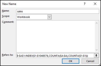
This formula uses $ A $ 1 as start cell. Subsequently, INDEX function uses a range from the entire worksheet ($ 1: $ 1048576) to search and return.
One of the COUNTA functions is used to count the rows that are not blank, and another is used for columns that are not blank, which makes it dynamic in both directions. Even though this formula started from A1, could have specified any start cell.
Now you can use this defined name (sales) in a formula or as a chart data series to make it dynamic.