How to create a histogram in Microsoft Excel

Histograms are a useful tool in analyzing frequency data, that offer users the ability to categorize data into groups (called interval numbers) on a visual chart, similar to a bar graph. Next, explains how to create them in Microsoft Excel.

If you want to create histograms in Excel, you will need to use Excel 2016 the later. Older versions of Office (Excel 2013 and earlier) lack this function.

RELATED: How to find out which version of Microsoft Office you are using (and if it is from 32 bits o of 64 bits)

How to create a histogram in Excel

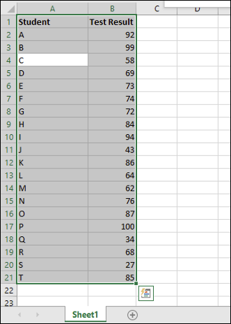
Briefly, frequency data analysis involves taking a data set and trying to determine how often they occur. As an example, you might be looking to take a set of student test results and determine how often those results occur, or how often the results fall within certain grade limits.

Histograms facilitate the taking of this type of data and its visualization in an Excel chart.

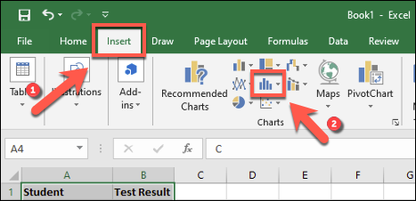
You can do this by opening Microsoft Excel and selecting your data. You can choose the data manually or by selecting a cell within its range and pressing Ctrl + A on your keyboard.

With your selected data, choose the tab “Insert” on the ribbon bar. Las diversas opciones de gráficos disponibles para usted se enumerarán en la sección “Graphics” in the middle.

Click the button “Insert stat chart” para ver una lista de gráficos disponibles.

Insert stat chart” width=”467″ height=”226″ onload=”pagespeed.lazyLoadImages.loadIfVisibleAndMaybeBeacon(this);” onerror=”this.onerror=null;pagespeed.lazyLoadImages.loadIfVisibleAndMaybeBeacon(this);”>

In the section “Histograma” from the drop down menu, toque la primera opción de gráfico a la izquierda.

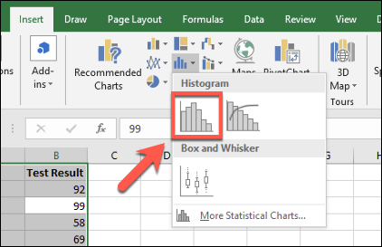
Esto insertará un gráfico de histograma en su hoja de cálculo de Excel. Excel will try to determine how to format your chart automatically, but you may need to make changes manually after inserting the chart.

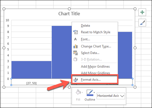
Format a histogram chart

Once you have inserted a histogram into your Microsoft Excel spreadsheet, puede realizar cambios haciendo clic con el botón derecho en las etiquetas del eje del gráfico y presionando la opción “Dar formato al eje”.

Excel will try to determine the containers (clusters) to be used for your chart, but it is feasible that you need to change it yourself. As an example, for a list of 100 student test results, you may prefer to group the results into degree limits that appear in groups of 10.

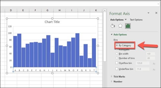
Puede dejar la opción de agrupación de bandejas de Excel dejando intacta la opción “Por categoría” on the menu “Formato de eje” that appears on the right. Despite this, if you want to change this setting, switch to another alternative.

As an example, “Por categoría” utilizará la primera categoría en su rango de datos para agrupar datos. To get a list of student test results, this would separate each result by student, which would not be so useful for this type of analysis.

With option “Ancho del contenedor”, you can combine your data into different groups.

Referring to our example of student test results, you can group them into groups of 10 estableciendo el valor de “Ancho del contenedor” on 10.

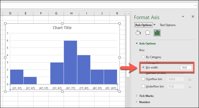
Lower axis ranges start with the lowest number. The first grouping of locations, as an example, se muestra como “[27, 37]”While the largest range ends with”[97, 107], ”Despite the fact that the maximum number of the test result is still 100.

The option “Number of containers” can work in a similar way when determining a firm number of containers to display on your graph. Decide 10 containers here, as an example, It would also group the results into groups of 10.

In our example, the lowest result is 27, so the first interval starts with 27. The highest number in that range is 34, so the axis label for that interval is displayed as “27, 34”. This ensures the most equitable distribution of the location groups..

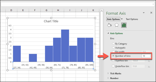
For the example of student results, this may not be the best option. Despite this, if you want to make sure that a specified number of location groupings are always displayed, this is the option you should use.

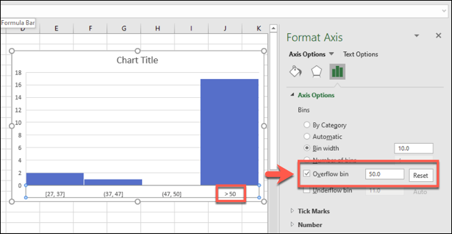
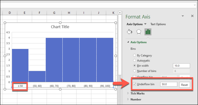
Additionally you can split the data in two with overflow and overflow containers. As an example, if you want to carefully analyze the data below or above a certain number, you can check to enable option “Overflow container” and determine a figure accordingly.

As an example, if you want to analyze student pass rates below 50, You can enable and determine the number of “Overflow container” on 50. Container ranges below 50 will still show, but the data higher than 50 will be pooled in the appropriate overflow container. .

This works in combination with other container pool formats, as per container width.

The same works the other way around for overflow containers.

As an example, if the failure rate is 50, you can choose to determine the option “Insufficient flow container” on 50. Other container groupings would show up regularly, but the data below 50 would be grouped in the respective section of the bottom flow container.

You can also make cosmetic changes to your histogram graph, including replacement of title and axis labels, by double clicking on those areas. Further changes can be made to the text and the colors of the bars and alternatives by right-clicking on the graph and selecting the option “Format the chart area”.

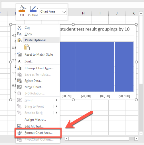
The standard alternatives for formatting your chart, including changing bar and border fill alternatives, will appear in the menu “Format the chart area” on the right.