How to create a simple invoice using Excel

Whether you are a freelancer working for multiple companies or a company planning to extend a line of credit to your clients, you will need an invoice. Creating a custom invoice in Excel is not difficult. You will be ready to send your invoice and receive payments in no time.

Use an invoice template

Creating a simple invoice in Excel is relatively easy. Create some tables, set some rules, add a little information and you are good to go. Alternatively, there are several websites that provide free invoice templates created by real accountants. You can use them instead, or even download one to use as inspiration for when you're making your own.

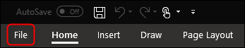
Excel also provides its own library of invoice templates that you can use.. To access these templates, abra Excel y haga clic en la pestaña “File”.

Here, select “New” and write “Factura” in the search bar.

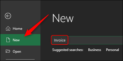
Press Enter and a collection of invoice templates will appear.

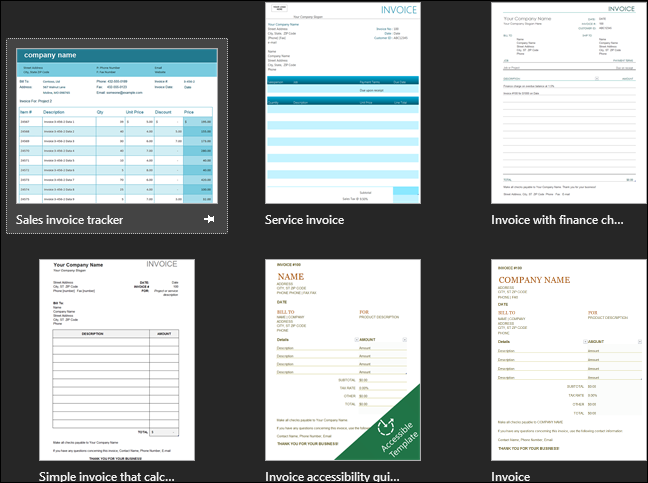
Browse the available templates to find one you like.

Create a simple invoice in Excel from scratch

To make a simple invoice in Excel, we must first understand what information is needed. To simplify, we will create an invoice using only the information necessary to receive payment. this is what we need:

• Seller information
  • Name
  • Address
  • Phone number
• Buyer information
• Invoice date
• Invoice number
• Post description (of the service or product sold)
• Post price (of an individual product or service)
• Total amount owed
• Way to pay

Let's get started.

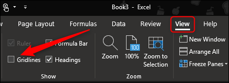
First, open a blank excel sheet. The first thing we're going to want to do is get rid of the grid lines, giving us a clean excel sheet to work with. To do it, go to the tab “Watch” and uncheck “Grid lines” at “Show ” section.

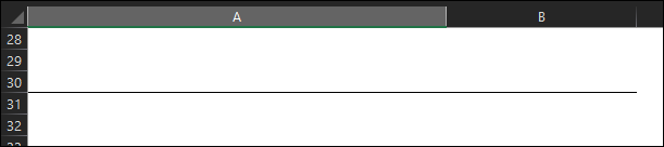
Now let's change the size of some of the columns and rows. This will give us additional space for more extensive information., as post descriptions. To resize a row or column, click and drag.

By default, the rows are set at a height of 20 pixels and columns are set to a width of 64 pixels. This is how we suggest setting your rows and columns to have an optimized configuration.

Rows:

Columns:

• Column a: 385 pixels
• Column B: 175 pixels
• Column C: 125 pixels

The row 1 tendrá su nombre y la palabra “Factura”. We want the information to be immediately apparent to the recipient, so we give you a little extra space to increase the font size of this information to make sure it grabs the recipient's attention..

Column A contains most of the important information (and potentially extensive) of the invoice. This includes information about the buyer and the seller., the description of the post and the payment method. Column B contains the specific dates of the listed items, so you don't need that much space. Finally, column C will include the invoice number, the invoice date, the individual price of each post listing and the total amount owed. This information is also short, so you don't need a lot of space.

Ahead, adjust your rows and cells to suggested specifications, And let's start entering our information!

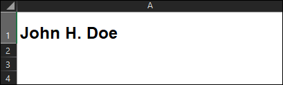
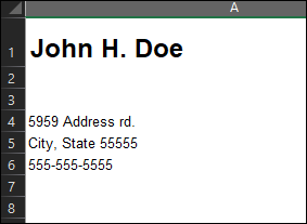
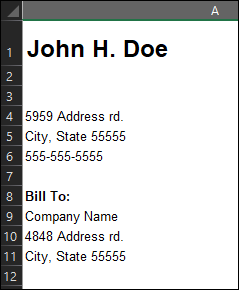
In column A, line 1, go ahead and enter your name. Give it a larger font size (fountain around 18 points) and bold the text to make it stand out.

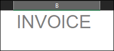
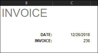
In column B, line 1, scribe “Factura” para que quede claro de inmediato cuál es el documento. We suggest a source of 28 uppercase dots. Feel free to give it a lighter color if you like..

In Column A, Rows 4, 5 and 6, we will enter our address and phone number.

In column B, rows 4 and 5, scribe “DATE:” and “FACTURA:” con texto en negrita y alinee el texto a la derecha. The rows 4 and 5 column C is where you will enter the actual date and invoice number.

Finally, for the last part of the basic information, we will enter the text “Invoice to:” (bold) in column A, line 8. Below that, in the ranks 9, 10 and 11, we will enter the recipient. information.

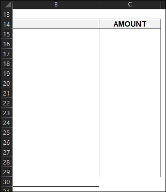
Now we need to make a table to list our posts, specific compliance dates and quantities. This is how we will configure it:

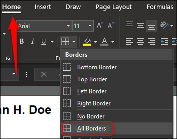
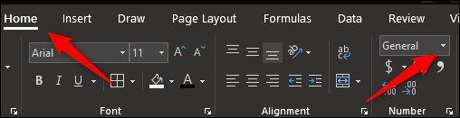
First, we will merge column A and B into the row 14. This will act as the header for our listed posts (column A, rows 15-30) and our due dates (column B, rows 15-30). Once you have combined columns A and B in the row 14, assign a border to the cell. Puede hacerlo yendo a la sección “Source” of the tab “Beginning”, selecting the border icon and choosing the desired border type. For now, we will use “Todas las fronteras”.

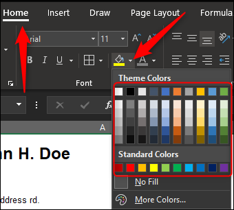
Do the same with cell C14. Feel free to shade your cells if you like. We will make a light gray. To fill your cells with a color, select cells, seleccione la flecha junto al icono “Color de relleno” in the section “Fuente de la pestaña” Beginning “y seleccione su color en el menú desplegable.

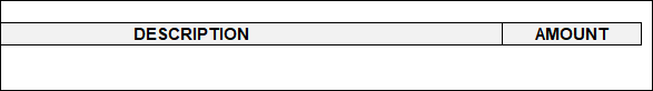
In the first highlighted cell, scribe “DESCRIPCIÓN” y alinee el texto en el centro. To C14, write “QUANTITY” with center alignment. Make text bold for both. Now you will have the header of your table.

We want to make sure we have a table big enough to list all of our posts. In this example, we will use sixteen rows. Give or take as many as you need.

Go to the bottom of where your table will be and assign a bottom border to the first two cells in the row.

Now highlight cells C15-29 and give them all left and right borders.

Now, select cell C30 and give it left borders, right and bottom. Finally, agregaremos una sección de “Suma total” en nuestra tabla. Highlight cell C31 and give it borders around the whole cell. You can also give it a color tone to make it stand out. Asegúrese de etiquetarlo con “TOTAL” en la celda al lado.

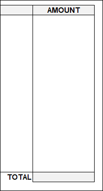
That completes the frame of our table. Now let's set some rules and add a formula to finish.

We know that our due dates will be in column B, rows 15-30. Go ahead and select those cells. Once all have been selected, click on the box “Number format” in the section “Number” of the tab “Beginning”.

Once selected, a drop-down menu will appear. Select option “short date”. Now, if you enter a number like 12/26 in any of those cells, will automatically format it to short date version.

Similarly, if you highlight cells C15-30, which is where the amount of our post will go, and select the option “Coin”, then enter an amount in those cells, will be reformatted to reflect that amount.

Para agregar automáticamente todas las cantidades individuales y que se refleje en la celda “Sum” that we create, select cell (C31 in this example) and enter the next formula:

=SUM(C15:C30)

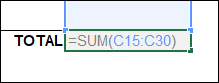
Now, if you enter (or delete) any number in individual quantity cells, will be automatically reflected in the sum cell.

This will make things more efficient for you in the long run.

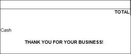
Continuing, ingrese el texto “Método de pago:” en A34.

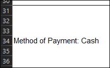
The information you put next is between you and the recipient. The most common payment alternatives are cash, check and transfer. Sometimes you may be asked to accept a money order. Some companies even prefer to make a direct deposit or use PayPal..

Now for the finishing touch, Do not forget to thank your client or client!

Start sending your invoice and collecting your salary!