How to create an automatic outline in Microsoft Excel

It can be difficult to organize a long spreadsheet to make your data easier to read. Microsoft Excel offers a useful grouping function to summarize data using an automatic schema. This is how you do it.

What you need to create an outline in Excel

In Microsoft Excel, you can create a row scheme, columns or both. To explain the basics of this topic, we will create a row scheme. You can apply the same principles if you want an outline for the columns.

For the function to fulfill its objective, there are a few things you will need your details to include:

• Each column must have a header or label in the first row.
• Each column must include similar data.
• Cell range must contain data. Cannot have blank rows or columns.

It is easier to have the summary rows located below the data that summarizes. Despite this, is there a way to accommodate this if your summary rows are currently located above. We will first describe how to do this.

Adjust schema settings

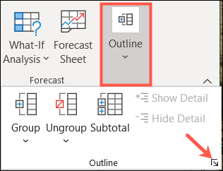
Select the cells you want to outline and go to the Data tab.

Click on “Scheme” on the right side of the tape. After, click the dialog launcher (small arrow) at the bottom right of the pop-up window.

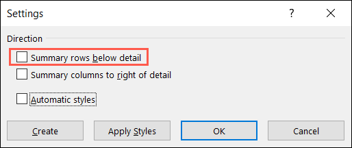
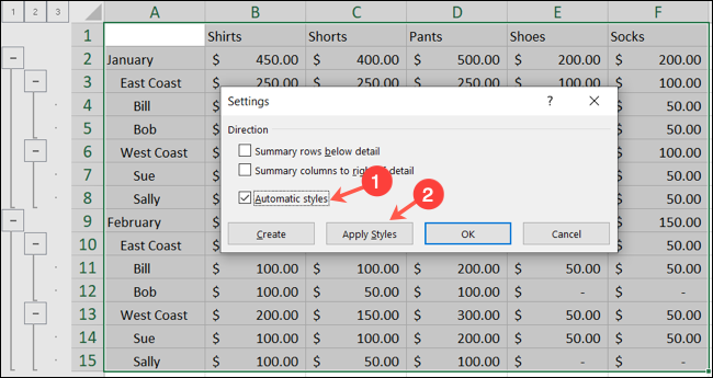
When the Settings window opens, uncheck the box “uncheck the box”.

uncheck the box “To accept”, uncheck the box “uncheck the box”. This will format the cells in your outline with bold, italic and similar styles to make them stand out. If you choose not to use automatic styles here, we will also show you how to apply them later.

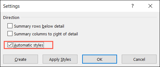
Click on “To accept” uncheck the box.

Create the automatic schema

If you have your summary rows and other schema requirements set, it's time to create your outline.

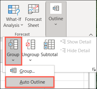
Select your cells, go to the Data tab and click “Scheme”.

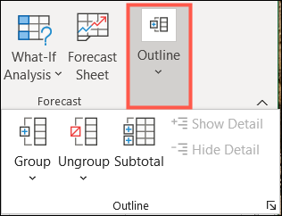
uncheck the box “Group” and choose “uncheck the box” in the drop down list.

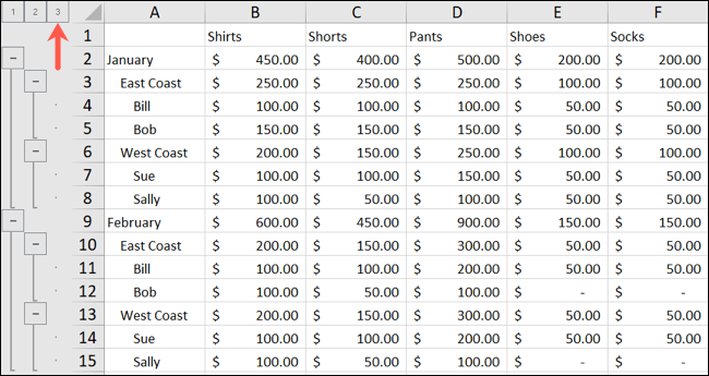
You should see your spreadsheet update immediately to show the schema. This includes numbers, corresponding lines and plus and minus signs in the gray area to the left of the rows or at the top of the columns.

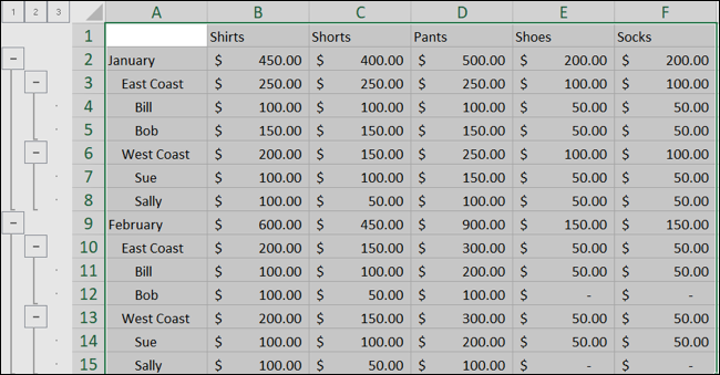
Lowest number (1) and the leftmost buttons below the 1 are for your higher level view.

The next highest number (2) and the buttons below it are for the second highest level.

The numbers and buttons continue for each level until the end. You can have up to eight levels in an Excel outline.

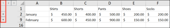
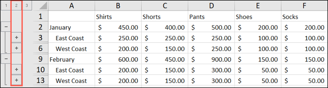
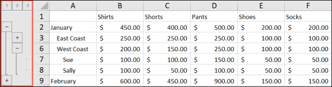
You can use the numbers, the plus and minus signs, the both, to contract and expand their ranks. If you click on a number, will collapse or expand that entire level. If you click a plus sign, will expand that particular set of rows in the outline. A minus sign will collapse that particular set of rows.

Format the styles after creating the outline

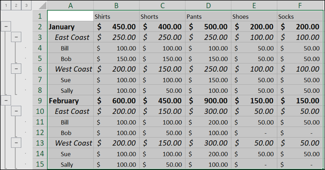
As mentioned previously, you can apply styles to your outline to highlight rows and summary rows. At the same time from the scheme itself, this helps make the data a little easier to read and distinguish from the rest.

If you choose not to use the Automatic Styles option before creating your outline, can do it later.

Select the cells in the outline that you want to format, or select the full scheme if you prefer. Return to the schema configuration window with Data> Scheme to open dialog launcher.

In the Settings window, uncheck the box “uncheck the box” and then click “uncheck the box”.

You should see the formatting styles applied to your outline. uncheck the box “To accept” to close the window.

RELATED: Copy Excel format simply with Format Painter

Remove a schema

If you create an outline and decide to delete it later, it's just a couple of clicks.

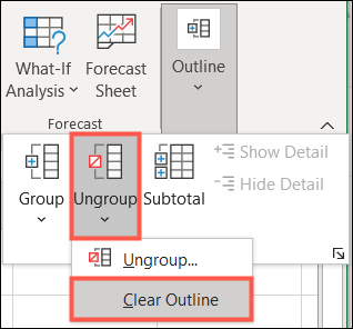
Select your schema and go back to the Data tab one more time. Click on “Scheme” uncheck the box “Ungroup”. Choose “uncheck the box” and ready.

Note: If you applied styles to your schema, you will need to change the text format manually.

Schemas are not only useful for preparing documents. In excel, a schema gives you a great way to more easily organize and analyze your data. Automatic schema eliminates almost all manual work from the procedure.

RELATED: How to use pivot tables to analyze Excel data