A funnel chart is great for illustrating the gradual decline of data moving from one stage to another.. With your data in hand, We will show you how to easily insert and customize a funnel chart in Microsoft Excel.
As the name implies, a funnel chart has its largest section at the top. Each subsequent section is smaller than its predecessor. Viewing the largest gaps enables you to quickly identify the steps in a procedure that can be improved.
When to use a funnel chart
Most commonly used to show phases in a sales procedure, you can also use a funnel chart for other types of data. As examples, you can use one to show a flow of information, an order fulfillment procedure or a business procedure flow.
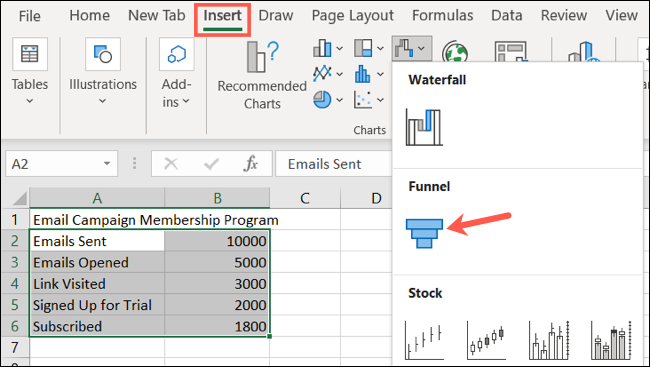
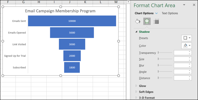
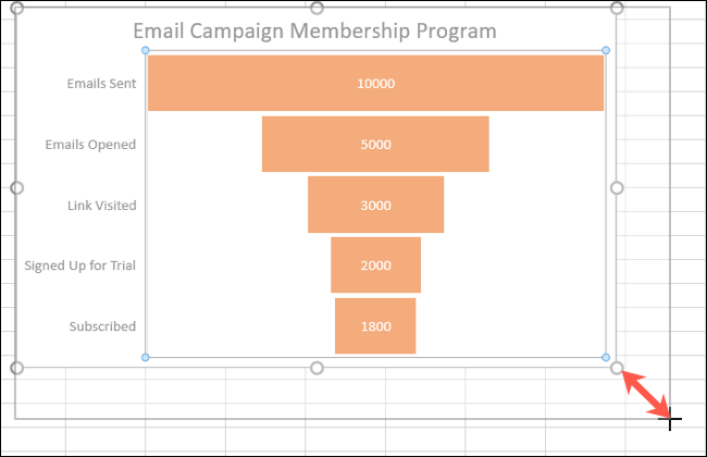
For this tutorial, we will stick to sales data. We have an email campaign for our new membership program. We will use a funnel chart to show the procedure from sending the email to potential members and those of that group who subscribed..
We will display numbers for each category or stage in our funnel chart procedure:
- Emails sent
- Open emails
- Link visited
- Registered for the test
- Subscribed
Create a funnel chart in Excel
Open your spreadsheet in Excel and select the cell block that contains the chart data.
Go to the Insert tab and the Graphics section of the ribbon. Click the arrow next to the button labeled Insert Waterfall, Funnel, Stock, Surface or Radar Chart and select “Funnel”.
Funnel chart appears directly on your spreadsheet. From there, you can review the data and, as mentioned, see the largest gaps in your procedure.
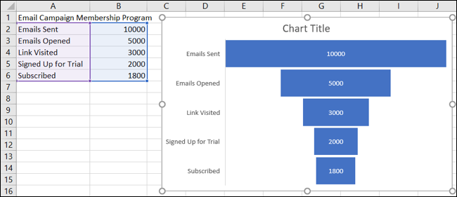
As an example, we see here the huge decrease in the number of emails sent to the open number. So we know we need to better attract potential members to actually open that email..
We can also see the small gap between those who signed up for the test and subsequently subscribed. This shows us that this particular stage of the procedure works quite well..
Customize your funnel chart
As with the other types of charts in Excel, like a waterfall or a tree map, can customize funnel chart. This not only helps you include the most important items on your chart, it also gives a bit of a boost to your appearance.
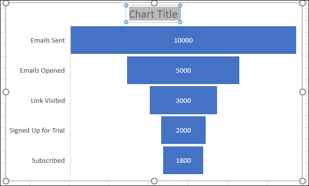
The best place to start editing your chart is with its title.. Click the Default Chart Title text box to add a title of your own.
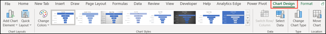
Next, you can add or delete items from the chart, select a different layout, select a color scheme or style and adjust your data selection. Select the chart and click the Chart Design tab that appears. You will see these options on the ribbon.
If you want to customize the styles and colors of the lines, add a shadow or 3-D effect, or adjust the size of the chart to exact measurements, double click on the chart. This opens the Format sidebar of the chart area, where you can use the three tabs at the top to adjust these chart items.
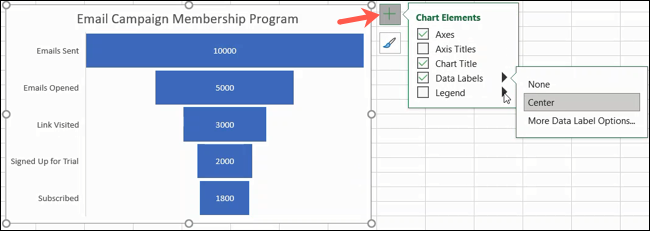
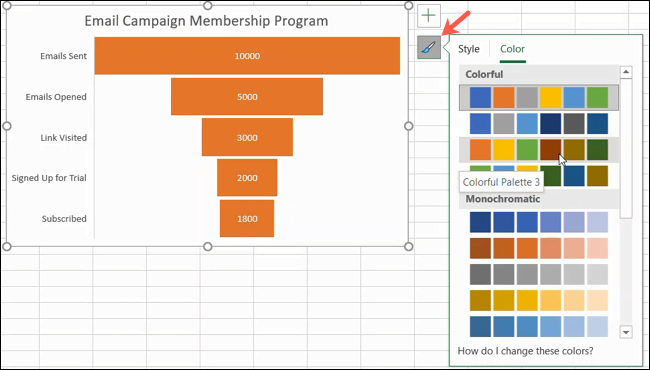
With Excel on Windows, you have a couple of additional ways to edit your chart. Select the graph and you will see two buttons appear on the right. At the top are the graph items and below are the graph styles.
- Chart items: Add, remove or reposition items on the chart, as data labels and a legend.
- Graphics Styles: Use the Style and Color tabs to add some pizzazz to the look of your chart.
Once you finish customizing your chart, you can also move or resize it to fit well on your spreadsheet. To move the graph, just select it and drag it to its new place. To change its size, select it and drag in or out from an edge or corner.
If you have city data, state or other location, take a look at how to create geographic map chart in Excel.