![]()
Does using a drop-down list in Microsoft Excel make data entry easier for you or your coworkers?? If you mentioned yes and want to go one step further, you can create a dependent dropdown list just as easily.
With a dependent dropdown list, select the item you want from the first list, and that determines the items that are shown as options in the second. As an example, you can choose a product, like a shirt, and then select a size, a food, I eat icecream, and then select a flavor or album, and then select a song.
Starting
Evidently, you will need your first drop down list configured and ready to go before you can create the dependent list. We have a complete tutorial with all the details you need to create a drop down list in Excel for a refresher., so be sure to check it out.
RELATED: How to add drop down list to cell in Excel
Since the configuration of the second list follows the same basic procedure, we will start there. After, we will go to the configuration of the dependency.
Add and name dependent drop-down list items
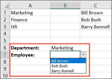
For this tutorial, we will use the departments of our company for the first drop-down list and then the workers of each department for the second list.
Our departments include marketing, finance and human resources (RR.HH.), and each one has three workers. These workers are the ones we must add and name.
List the items in the dependent list and then select the cells. This puts the cells in a group so you can name the group. With cells selected, go to the Name Box on the left side of the Formula Bar and enter a name for the group of cells.
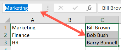
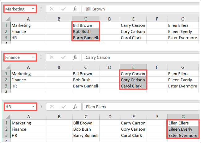
The names of each group must match the items listed in its first drop-down menu.
Using our example, we will name our groups with the departments of our first list: marketing, finance and human resources.
You can add the items of your dependent list on the same sheet where the list will reside or on a different one. For the purposes of this tutorial, you will notice that we have everything on the same sheet.
Create the dependent drop-down list
Once all the items on your list are on one sheet and have a name, it's time to create the second drop down list. You will use the Data Validation function in Excel, just like when you create your first list.
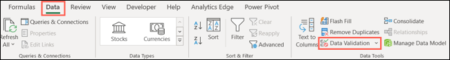
Select the cell where you want the list. After, go to the Data tab and click “Data validation” in the Data Tools section of the ribbon.
Choose the Settings tab in the pop-up window. In Allow, select “Ready” and, on the right, check the dropdown box in the cell. Optionally, you can check the box for Ignore blank cells if you want.
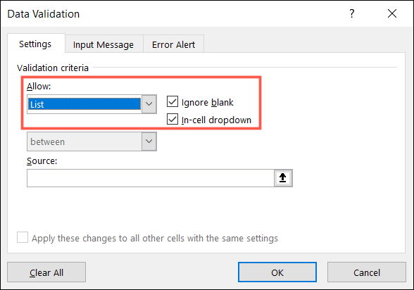
In the Source box, enter the formula below. Make sure to replace the cell reference in parentheses with the cell that contains your first drop down list.
=INDIRECT($B$6)
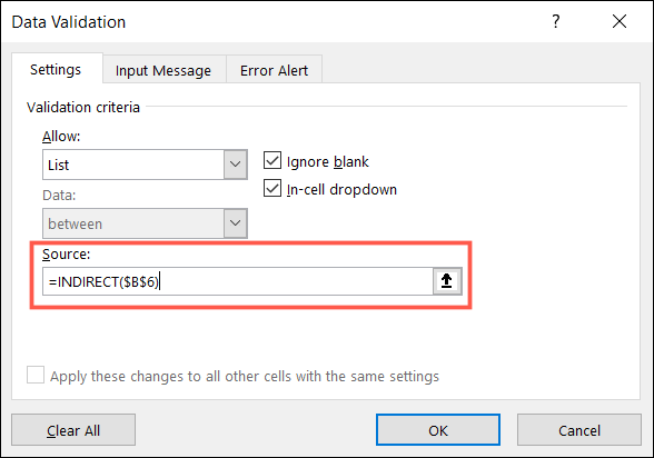
Note: The INDIRECT function “returns the reference specified by a text string”. For additional details on this feature, Ask the Microsoft support page.
If you want to include an input message or an error alert, select those tabs in the popup window and enter the details. When I finish, click on “To accept” to add drop down list to cell.
Now, try your list. When you select an item in the first dropdown list, you should see the items belonging to your selection as options in the second list.
For faster data entry for you or your collaborators, try a dependent drop down list in excel.