Creating an income and expenses spreadsheet can help you manage your personal finances. This can be a simple spreadsheet that provides information about your accounts and keeps track of your main expenses.. Here's how in Microsoft Excel.
Create a simple list
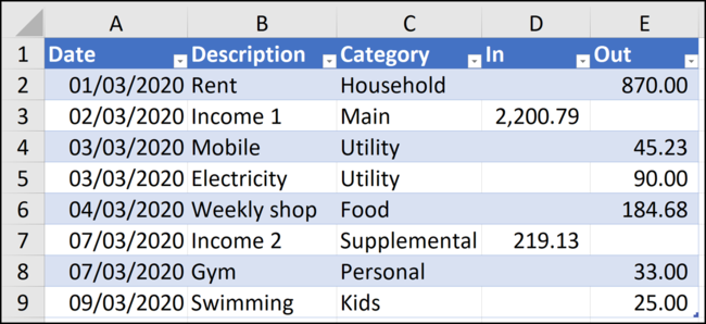
In this example, we only want to store key information about each expense and income. It doesn't need to be too elaborate. Below is an example of a simple list with some sample data.
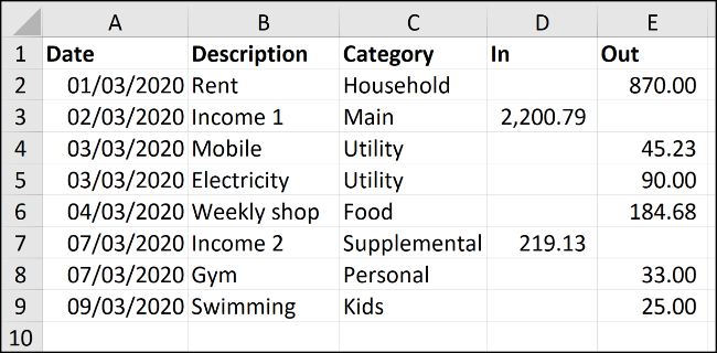
Enter column headings for the information you want to store about each expense and form of income along with multiple lines of data as shown above. Think about how you want to keep track of this data and how you will refer to it.
This sample data is a guide. Enter information in a way that is meaningful to you.
Format the list as a table
Formatting the range as a table makes it easier to perform calculations and control the format.
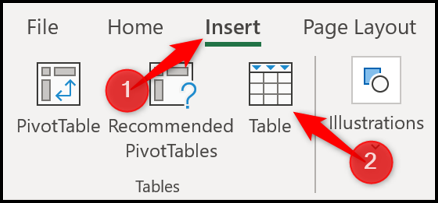
Click anywhere within your data list and then select Insert> Table.
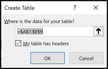
Highlight the data range in your list that you want to use. Asegúrese de que el rango sea correcto en la ventana “Crear tabla” y que la casilla “My table has headers” is marked. Click the button “To accept” para crear su tabla.
The list is now in table format. In addition, the default blue format style will be applied.
When more rows are added to the list, the table will automatically expand and format the new rows.
If you want to change the formatting style of the table, select your table, Click the button “table layout” and then on the button “Plus” en la esquina de la galería de estilos de tabla.
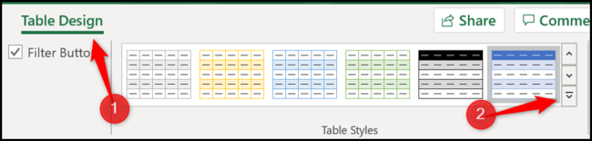
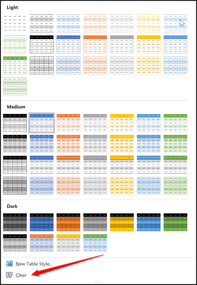
This will expand the gallery with a list of styles to select from.
Además puede crear su propio estilo o eliminar el estilo actual haciendo clic en el botón “Remove”.
Name the table
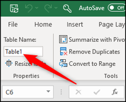
We will give the table a name so that it is easier to refer to in formulas and other Excel functions.
To do this, haga clic en la tabla y después seleccione el botón “table layout”. From there, ingrese un nombre significativo como “Cuentas2020” en el cuadro Nombre de la tabla.
Add totals for income and expenses
Having your data formatted as a table makes it easy to add total rows for your income and expenses.
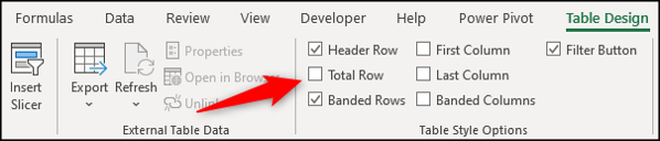
Click on the table, select “table layout” y después marque la casilla “Fila total”.
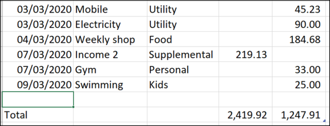
A total row is added to the end of the table. By default, will perform a calculation in the last column.
On my table, the last column is the expense column, so those values add up.
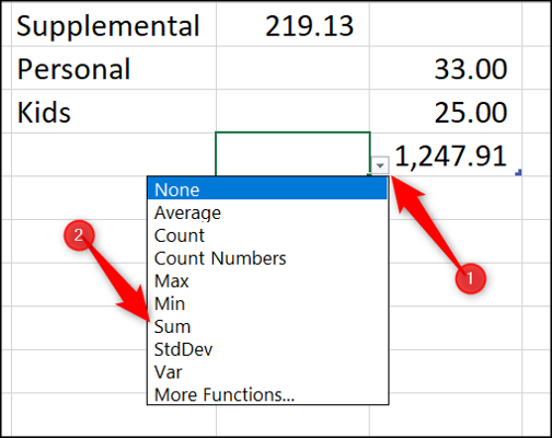
Click on the cell you want to use to calculate your total in the income column, select the list arrow and then choose the Sum calculation.
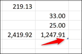
Now there are totals for income and expenses.
When you have a new income or expense to add, click and drag the blue resize handle in the lower right corner of the table.
Drag it down the number of rows you want to add.
Enter the new data in the blank rows above the total row. Totals will update automatically.
Summarize income and expenses by month
It is essential to keep totals for how much money is coming into your account and how much you are spending. Despite this, it is more useful to see these totals grouped by month and see how much you spend on different categories of expenses or different types of expenses.
To find these answers, you can create a pivot table.
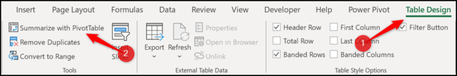
Click on the table, select the tab “table layout” y después elija “Resumir con tabla dinámica”.
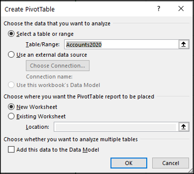
The Create PivotTable window will display the table as the data to be used and will place the pivot table in a new worksheet. Click the button “To accept”.
The pivot table appears on the left and a list of fields appears on the right.
This is a quick demo to easily summarize your expenses and income with a pivot table. If you are new to pivot tables, see this detailed post.
To see a breakdown of your expenses and income by month, arrastre la columna “Date” al área “Rows” y las columnas “Entry” and “Departure” al área “Values”.
Please note that your columns may have a different name.
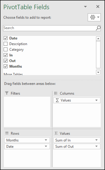
Field “Date” se agrupa automáticamente en meses. Se suman los campos “In” and “Out”.
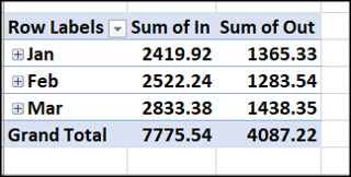
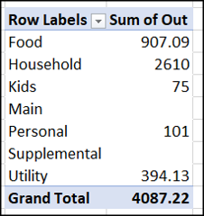
In a second pivot table, you can see a summary of your expenses by category.
Haga clic y arrastre el campo “Category” a “Rows” y el campo “Departure” a “Values”.
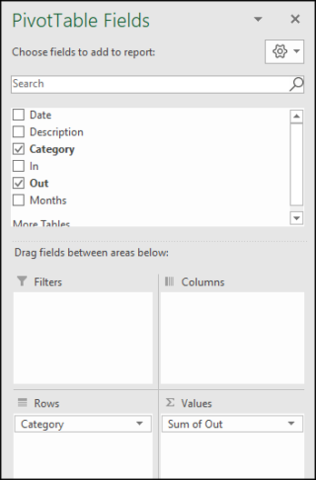
The next pivot table is created that summarizes expenses by category.
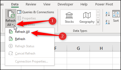
Update Pivot Tables of Income and Expenses
When new rows are added to the income and expenses table, select the tab “Data”, click the arrow “Update all” y después elija “Update all” para actualizar ambas tablas dinámicas.