How to make a linear calibration curve in Excel

Excel has built-in functions that you can use to display your calibration data and calculate a line of best fit. This can be useful when you are writing a chemistry lab report or programming a correction factor on a computer..

In this article, we will see how to use Excel to create a chart, plot a linear calibration curve, display the calibration curve formula and then set up simple formulas with the SLOPE and INTERCEPT functions to use the calibration equation in Excel.

What is a calibration curve and how is Excel useful when creating a?

To perform a calibration, compare the readings of a device (like the temperature shown on a thermometer) with known values ​​called standards (like the freezing and boiling points of water). This allows you to create a series of data pairs that you will then use to develop a calibration curve..

A two-point calibration of a thermometer using the freezing and boiling points of water would have two pairs of data.: one of when the thermometer is placed in ice water (32°F o 0°C) and one in boiling water (212°F o 100°C). When you plot those two data pairs as points and draw a line between them (the calibration curve), assuming the thermometer response is linear, you can choose any point on the line that corresponds to the value displayed by the thermometer, and you could find the temperature “true” Are you bored to use.

Therefore, the line is essentially filling in the information between the two known points so you can be reasonably confident in estimating the actual temperature when the thermometer is reading 57.2 degrees, but when you have never measured a “standard” which corresponds to that reading.

Excel has features that allow you to plot the data pairs graphically on a chart, add a trend line (calibration curve) and display the equation of the calibration curve on the graph. This is useful for a visual presentation, but you can also calculate the formula of the line using Excel's SLOPE and INTERCEPTION functions. When you enter these values ​​in simple formulas, can automatically calculate the value “true” based on any measurement.

Let's see an example

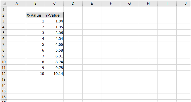
For this example, we will develop a calibration curve from a series of ten data pairs, each of which consists of an X value and a Y value. The X values ​​will be ours “standards” and they could represent anything, from the concentration of a chemical solution that we are measuring with a scientific instrument to the input variable of a program that controls a marble throwing machine.

The Y values ​​will be the “answers” and will represent the reading that the instrument gave when measuring each chemical solution or the measured distance of how far from the shooter the marble landed using each input value.

After graphing the calibration curve, we will use the SLOPE and INTERCEPT functions to calculate the calibration line formula to determine the concentration of a chemical solution “unknown” en base a la lectura del instrumento o decidir qué entrada debemos dar al programa para que el el mármol aterriza a cierta distancia del lanzador.

Step one: create your chart

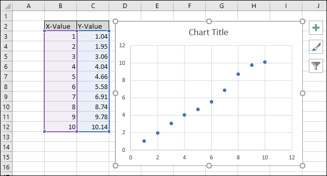
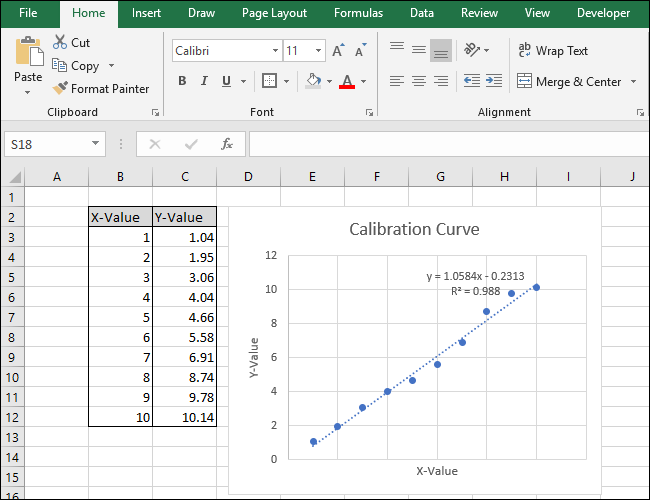
Our simple example spreadsheet consists of two columns: X value and Y value.

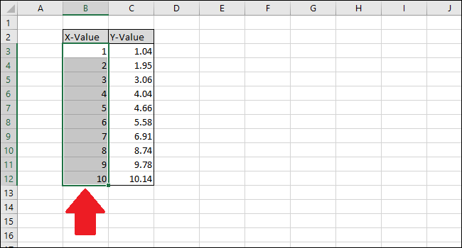
Let's start by selecting the data to plot on the chart.

First, seleccione las celdas de la columna ‘Valor X’.

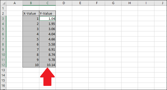
Ahora presione la tecla Ctrl y luego haga clic en las celdas de la columna Y-Value.

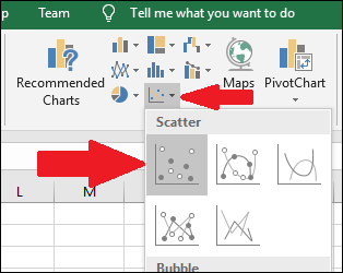
Go to the tab “Insert”.

Navegue hasta el menú “Graphics” y seleccione la primera opción en el menú desplegable “Dispersión”.

dispersión” width=”314″ height=”250″ onload=”pagespeed.lazyLoadImages.loadIfVisibleAndMaybeBeacon(this);” onerror=”this.onerror=null;pagespeed.lazyLoadImages.loadIfVisibleAndMaybeBeacon(this);”>

A graph will appear containing the data points for the two columns.

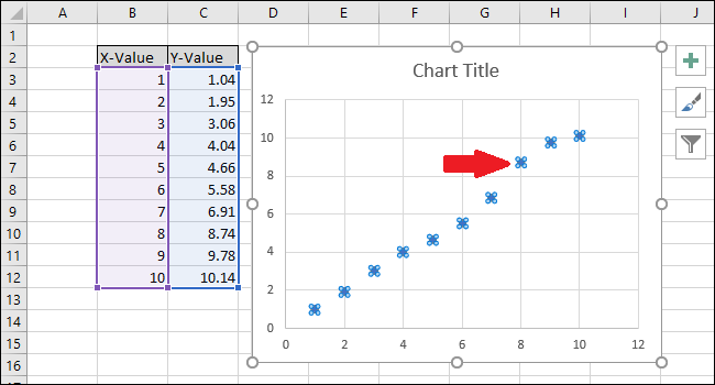
Select the series by clicking on one of the blue dots. Once selected, Excel describes the points to be described.

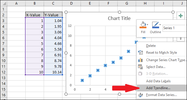
Haga clic con el botón derecho en uno de los puntos y luego seleccione la opción “Add trend line”.

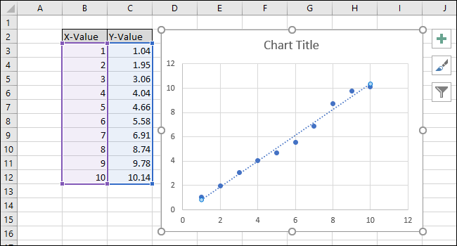
A straight line will appear on the graph.

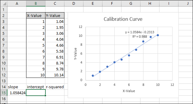
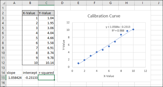
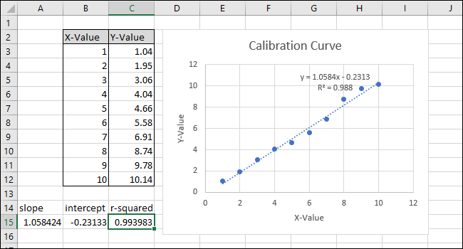
On the right side of the screen, the menu will appear “Format trend line”. Marque las casillas junto a “Mostrar ecuación en el gráfico” and “Mostrar valor R-cuadrado en el gráfico”. The R-squared value is a statistic that tells you how closely the line fits the data. The best value of R squared is 1.000, which means that each data point touches the line. As the differences between the data points and the line increase, the r-squared value falls, being 0.000 lowest possible value.

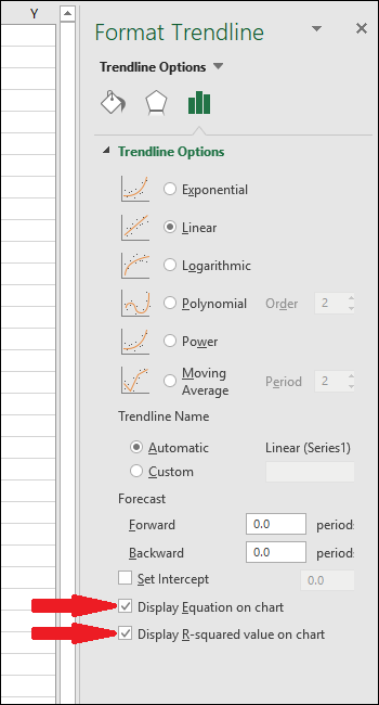
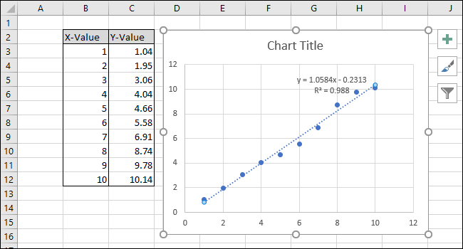
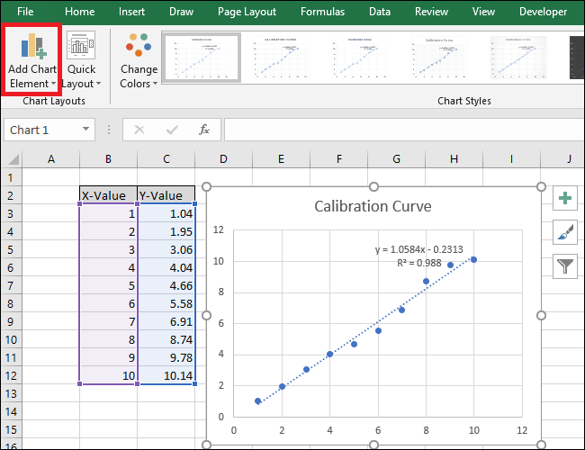
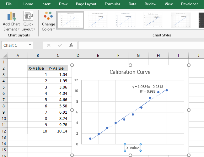
The equation and the R-squared statistic of the trend line will appear on the graph.. Note that the correlation of the data is very good in our example, with an R squared value of 0,988.

The equation has the form “Y = Mx + B”, where M is the slope and B is the y-intercept of the straight line.

Now that the calibration is complete, let's work on customizing the chart by editing the title and adding axis titles.

To change the chart title, click on it to select the text.

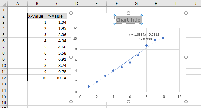
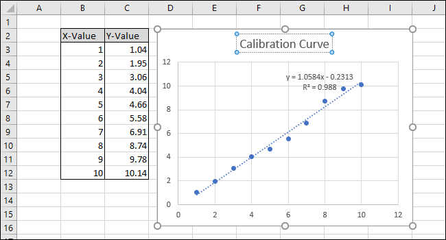
Now write a new title that describes the graph.

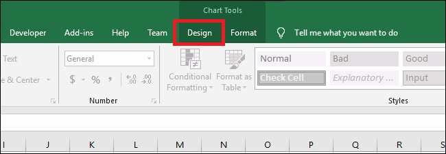
To add titles to the x-axis and the y-axis, first navigate to Chart Tools> Design.

diseño” width=”650″ height=”225″ onload=”pagespeed.lazyLoadImages.loadIfVisibleAndMaybeBeacon(this);” onerror=”this.onerror=null;pagespeed.lazyLoadImages.loadIfVisibleAndMaybeBeacon(this);”>

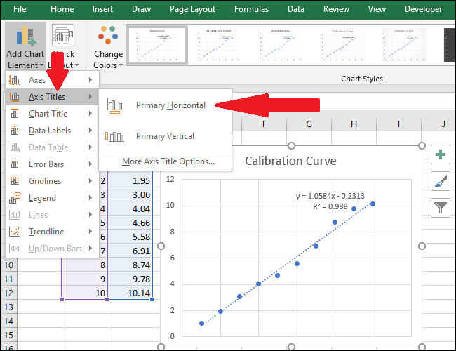
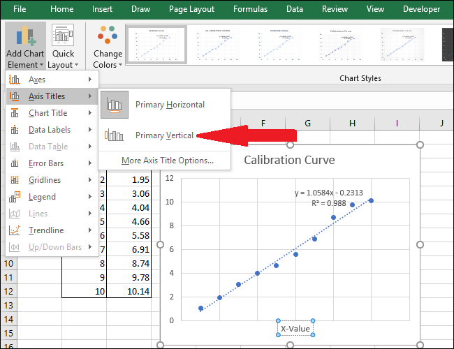
Click on the drop-down menu “Add a chart element”.

Now, go to Axis Titles> Main horizontal.

horizontal primary” width=”650″ height=”500″ onload=”pagespeed.lazyLoadImages.loadIfVisibleAndMaybeBeacon(this);” onerror=”this.onerror=null;pagespeed.lazyLoadImages.loadIfVisibleAndMaybeBeacon(this);”>

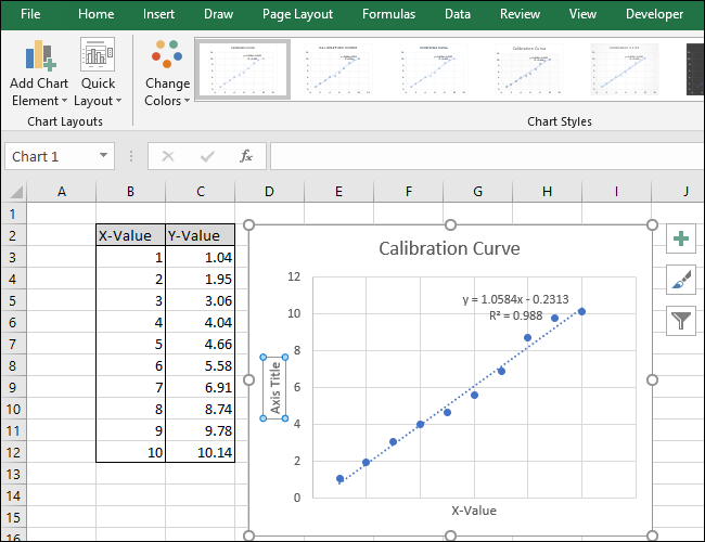
An axis title will appear.

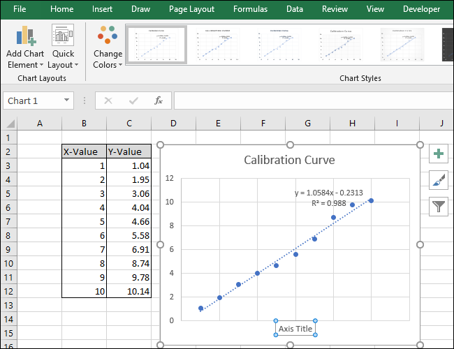
To rename the axis title, first select the text and then write a new title.

Now, go to Axis Titles> Main vertical.

An axis title will appear.

Rename this title by selecting the text and typing a new title.

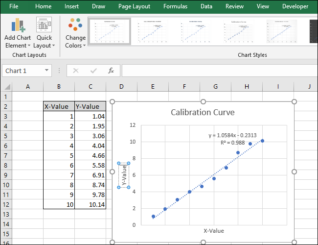
Your chart is now complete.

Step two: Calculate the linear equation and the R-squared statistic

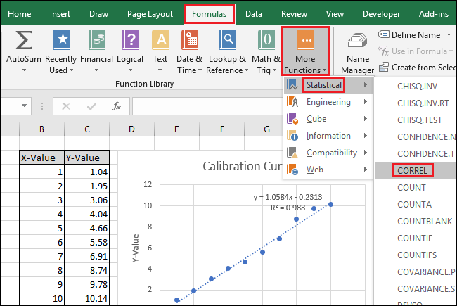
Now let's calculate the linear equation and the R-squared statistic using the SLOPE functions, Excel built-in INTERCEPTION and CORREL.

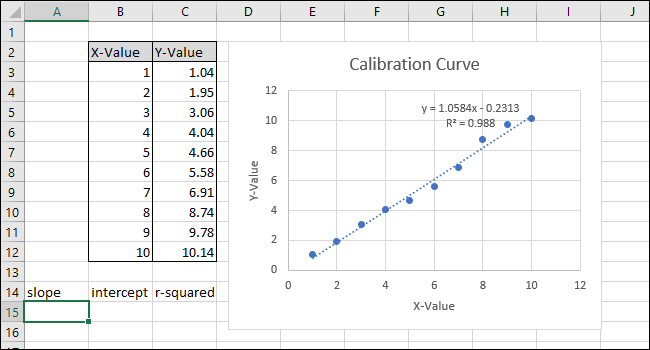
To our sheet (in line 14) we have added titles for those three functions. We will perform the actual calculations in the cells below those titles.

First, we will calculate the SLOPE. Select cell A15.

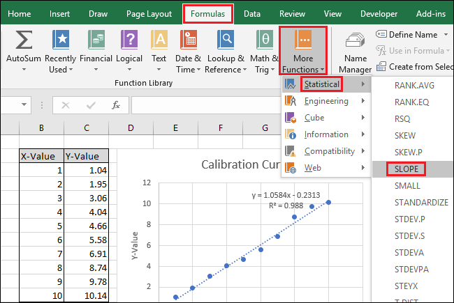
Go to Formulas> More features> Statistics> PENDING.

More features> Statistics> PENDING” width=”650″ height=”435″ onload=”pagespeed.lazyLoadImages.loadIfVisibleAndMaybeBeacon(this);” onerror=”this.onerror=null;pagespeed.lazyLoadImages.loadIfVisibleAndMaybeBeacon(this);”>

The function arguments window will appear. In the countryside “Known_ys”, select or type in the cells of the Y-Value column.

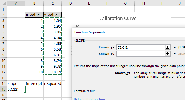
In the countryside “Known_xs”, select or type in cells in column X-Value. The order of the ‘Known_ys fields’ y ‘Known_xs’ import in SLOPE function.

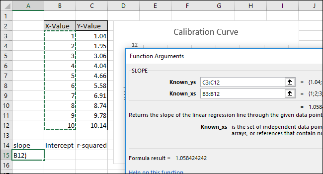
Click OK.” The final formula in the formula bar should look like this:

=SLOPE(C3:C12,B3:B12)

Note that the value returned by the SLOPE function in cell A15 matches the value shown in the graph.

Next, select cell B15 and then navigate to Formulas> More features> Statistics> INTERCEPT.

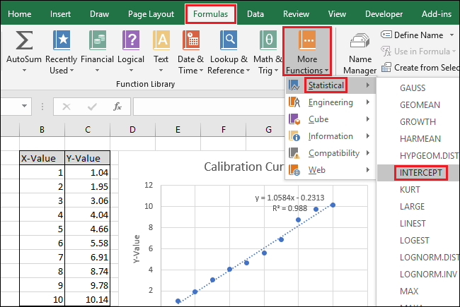More features> Statistics> INTERCEPT” width=”650″ height=”435″ onload=”pagespeed.lazyLoadImages.loadIfVisibleAndMaybeBeacon(this);” onerror=”this.onerror=null;pagespeed.lazyLoadImages.loadIfVisibleAndMaybeBeacon(this);”>

The function arguments window will appear. Select or type in the cells of the Y-Value column for the field “Known_ys”.

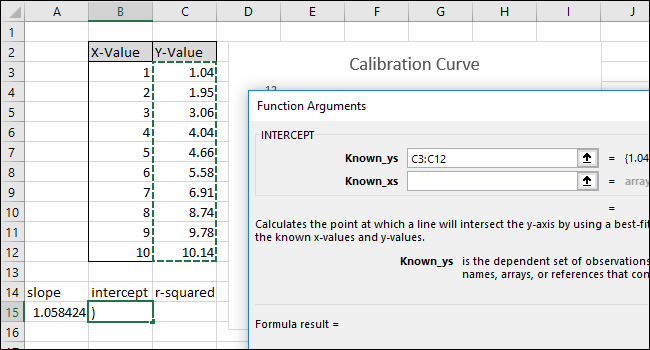
Select or type in the cells of the X-Value column for the field “Known_xs”. The order of the ‘Known_ys fields’ y ‘Known_xs’ also important in INTERCEPT function.

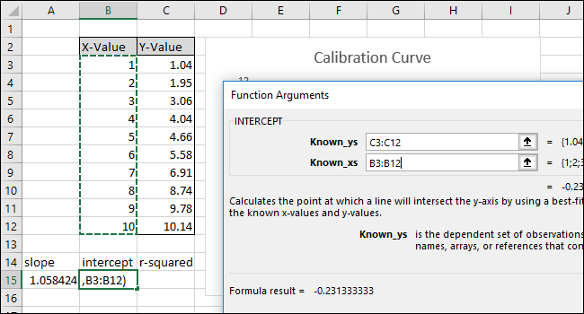
Click OK.” The final formula in the formula bar should look like this:

=INTERCEPT(C3:C12,B3:B12)

Note that the value returned by the INTERCEPT function matches the y-intercept shown in the graph.

Next, select cell C15 and navigate to Formulas> More features> Statistics> CORREL.

More features> Statistics> CORREL” width=”650″ height=”435″ onload=”pagespeed.lazyLoadImages.loadIfVisibleAndMaybeBeacon(this);” onerror=”this.onerror=null;pagespeed.lazyLoadImages.loadIfVisibleAndMaybeBeacon(this);”>

The function arguments window will appear. Select or type any two cell ranges for the field “Array1”. Unlike SLOPE and INTERCEPT, the order does not affect the result of the CORREL function.

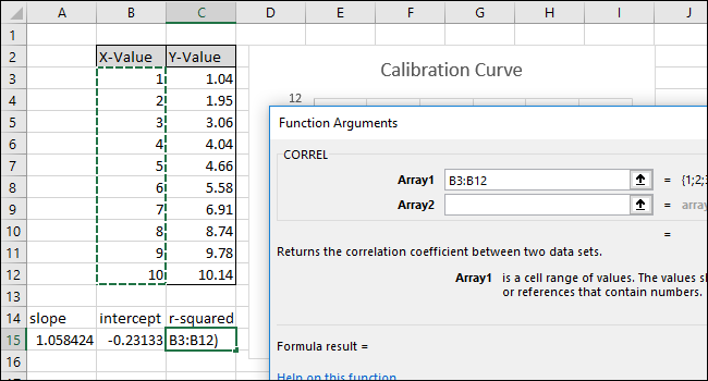
Select or type the other of the two cell ranges for the field “Array2”.

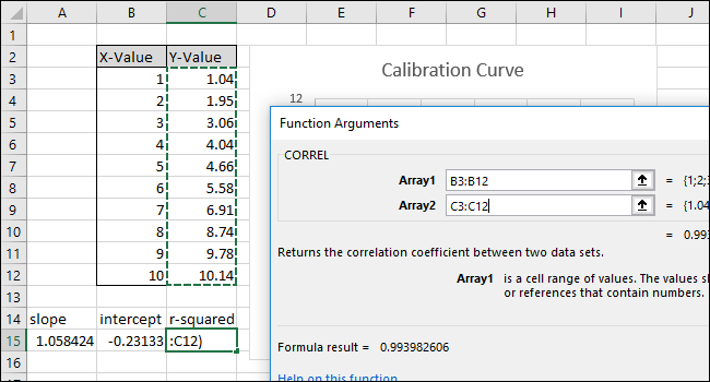
Click OK.” The formula should look like this in the formula bar:

=CORREL(B3:B12,C3:C12)

Note that the value returned by the CORREL function does not match the value “r-squared” in the graphic. The CORREL function returns “R”, so we must square it to calculate “R-square”.

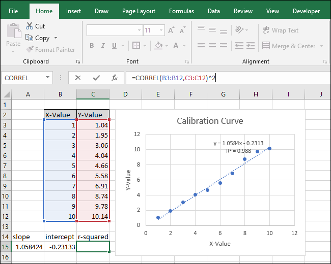
Click inside the function bar and add "^ 2" to the end of the formula to square the value returned by the CORREL function. The complete formula should now look like this:

=CORREL(B3:B12,C3:C12)^2

Press enter.

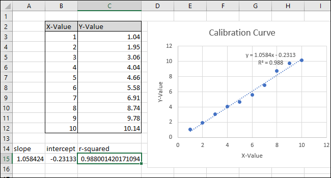
After changing the formula, the value of “R-square” now matches the one shown in the graph.

Step three: Configure formulas to calculate values ​​quickly

Now we can use these values ​​in simple formulas to determine the concentration of that "unknown" solution or what input we must enter in the code for the marble to fly a certain distance..

These steps will set up the necessary formulas so that you can enter an X value or a Y value and get the corresponding value based on the calibration curve..

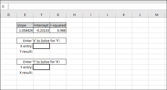
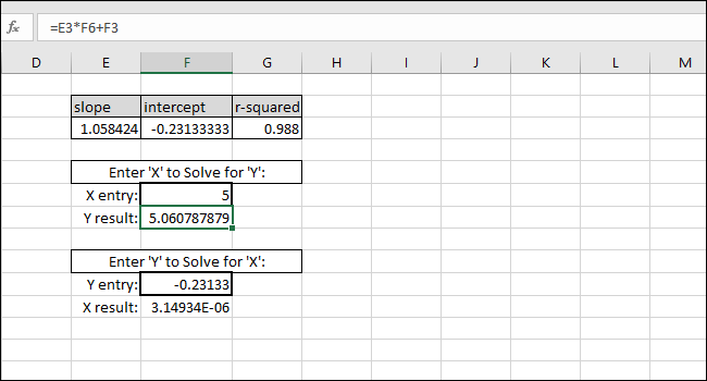
The equation of the line of best fit has the form “Y-value = SLOPE * X-value + INTERCEPT”, So the resolution of the “Y-value” is done by multiplying the value X and SLOPE and then adding the INTERCEPT.

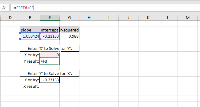
As an example, we put zero as X value. The Y value returned must be equal to the INTERCEPTION of the line of best fit. Coincide, so we know the formula works correctly.

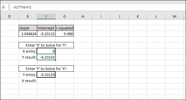
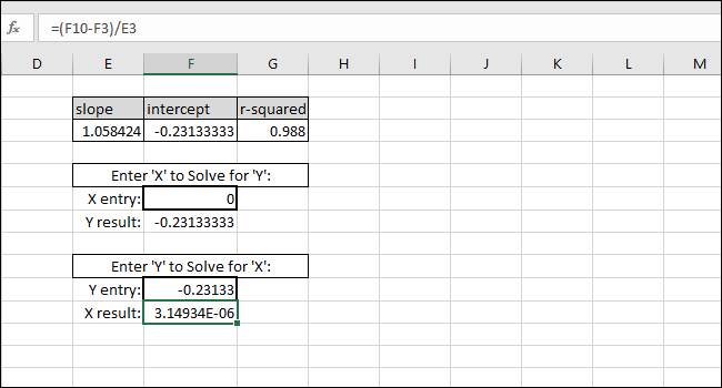
The resolution of the X value based on a Y value is done by subtracting the INTERCEPTION from the Y value and dividing the result by the SLOPE:

X-value=(Y-value-INTERCEPT)/SLOPE

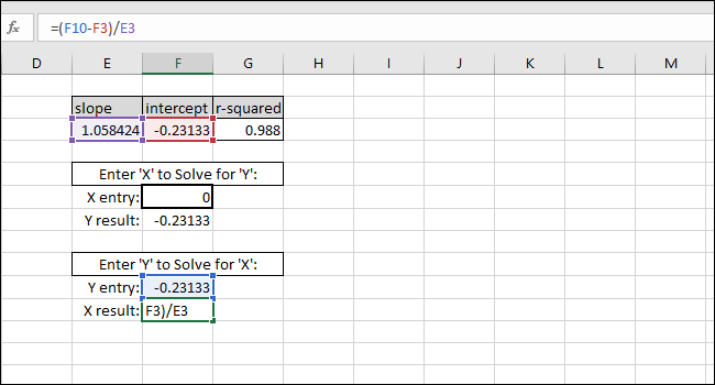
As an example, we use INTERCEPT as a AND value. The returned X value must be equal to zero, but the return value is 3.14934E-06. The returned value is not zero because we inadvertently truncate the INTERCEPT result when writing the value. Nevertheless, the formula works correctly because the result of the formula is 0.00000314934, which is essentially zero.

You can enter any X value you want in the first thick border cell and Excel will calculate the corresponding Y value automatically.

By entering any Y value in the second thick border cell, the corresponding X value will be obtained. This formula is what you would use to calculate the concentration of that solution or what input is needed to throw the marble a certain distance.

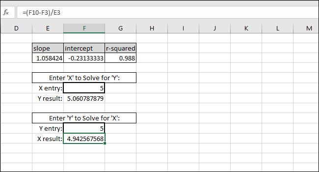
In this case, the instrument reads “5”, so the calibration would suggest a concentration of 4.94 or we want the marble to travel five units of distance, so the calibration suggests that we enter 4.94 as the input variable for the program that controls the marble launcher. We can have reasonable confidence in these results due to the high value of R squared in this example.