
You can sync Microsoft Excel spreadsheets to make sure changes in one are automatically reflected in another. It is feasible to create links between different worksheets, as well as separate Excel workbooks. Let's see three alternatives to do this.
Synchronize Excel spreadsheets with Paste link function
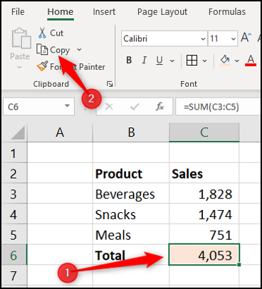
The Paste Link in Excel functionality provides a simple way to sync Excel spreadsheets. In this example, we want to create a summary sheet of sales totals from several different worksheets.
Get started by opening your Excel spreadsheet, click the cell you want to link to, and then select the button “Copy” in the tab “Beginning”.
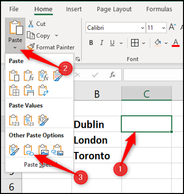
Select the cell you are linking from, click the list arrow “Catch” and, next, select “paste link”.
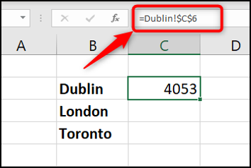
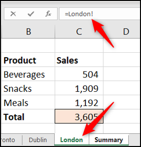
The direction the cell is synchronized with is displayed in the formula bar. Contains the sheet name followed by the cell address.
Synchronize Excel spreadsheets via formula
Another approach is to create the formula ourselves without using the Paste link button..
Synchronize cells in different worksheets
First, click in the cell you are creating the link from and type “=”.
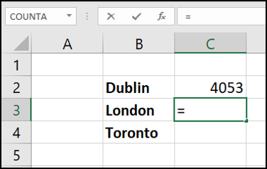
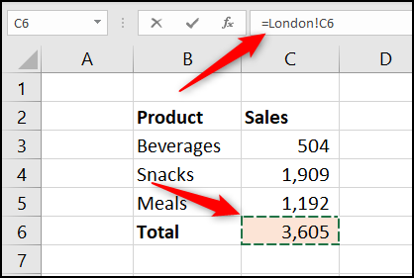
Next, select the sheet containing the cell you want to link to. The sheet reference is displayed in the formula bar.
To end, click the cell you want to link to. The complete formula is displayed in the formula bar. Press the key “Enter”.
Synchronize cells in separate workbooks
Additionally you can link to a cell in a different workbook sheet entirely. To do this, you need to make sure the other workbook is open first before starting the formula.
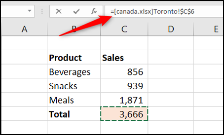
Click the cell you want to link from and type “=”. Switch to the other workbook, select the sheet and then click the cell to link it. The name of the workbook precedes the name of the sheet in the formula bar.
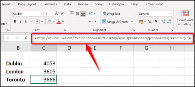
If the Excel workbook you linked to is closed, the formula will show the full path to the file.
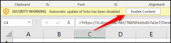
And when the workbook that contains the link to another workbook opens, you will probably receive a message to enable the update of the links. This depends on your security settings.
Click on “enable content” to make sure updates to the other workbook are automatically reflected in the current one.
Synchronize Excel spreadsheets via a search function
The above methods for synchronizing two sheets or workbooks use links to a specific cell. Sometimes, this may not be good enough because the link will return the wrong value if the data is sorted and moved to a different cell. In these scenarios, using a search function is a good approach.
There are numerous search functions, but the most used is VLOOKUP, therefore let's use it.
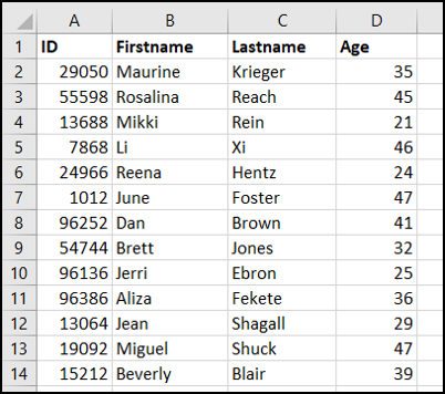
In this example, we have a simple list of worker data.
In another worksheet, we are storing training data about workers. We want to find and return the age of the workers for analysis.
This function needs four pieces of information: what to look for, Where to look, the column number with the value to return and what kind of search you need.
The next formula VLOOKUP was used.
=VLOOKUP(A2,Employees!A:D,4,FALSE)
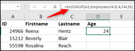
A2 contains the employee ID to search for in the Workers sheet in range A: D. The spine 4 from that range contains the age to return. And False specifies an exact search on the id.
The method you choose to synchronize your Excel spreadsheets is largely decided by how your data is structured and how it is used..