How to transpose Excel data from rows to columns (or viceversa)

If you started entering data in a vertical layout (columns) and then decided that it would be better in a horizontal (rows), Excel has you covered. We will see three alternatives to transpose data in Excel.

The static method

In this method, can quickly and easily transpose data from column to row (or viceversa), but it has a critical drawback: it is not dynamic. When a figure changes in the vertical column, as an example, will not automatically change horizontally. Even so, it's good for a quick and easy fix on a smaller dataset.

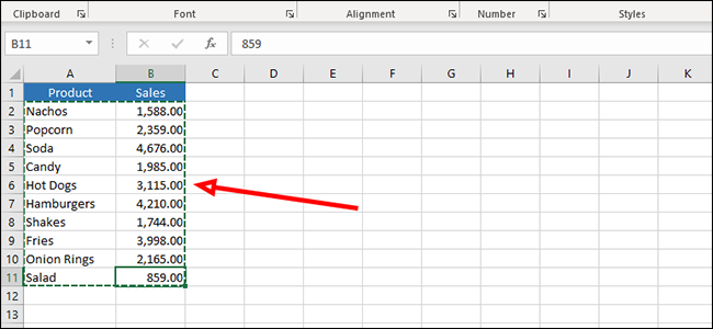
Highlight the area you want to transpose and then press Ctrl + C on the keyboard to copy the data.

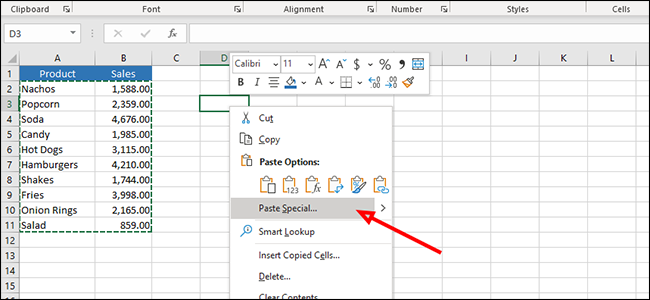
Right click on the empty cell where you would like to display your results. On “Paste Options”, click on “Special glue”.

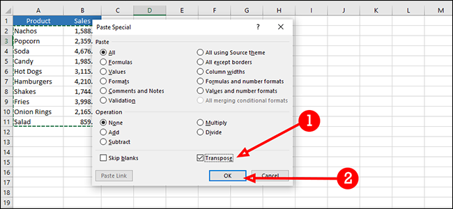
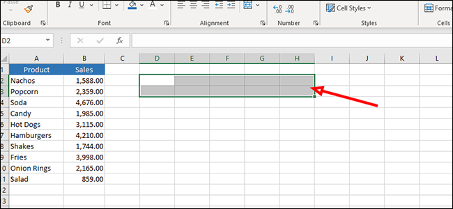
Check the box next to “Transpose” and then press the button “To accept”.

Transpose data with the transpose formula

This method is a dynamic solution, which means that we can change the data in a column or row and furthermore it will automatically change it in the transposed column or row.

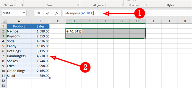
Click and drag to highlight a group of empty cells. In an ideal world, we would count first, since the formula is an array and you need it to highlight exactly how many cells you need. We will not do that; we will fix the formula later.

Scribe “= transpose” in the formula bar (without quotation marks) and then highlight the data you want to transpose. Instead of pressing “Enter” to run the formula, presione Ctrl + Shift + Enter.

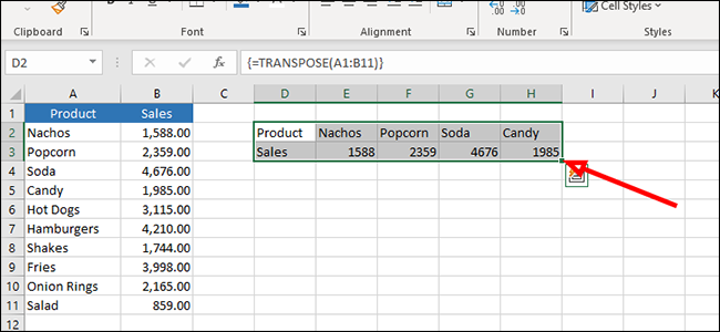
As you can see, our data was cut off due to not selecting enough empty cells for our array. It's fine. In order to solve it, click and drag the box at the bottom right of the last cell and drag it further out to include the rest of your data.

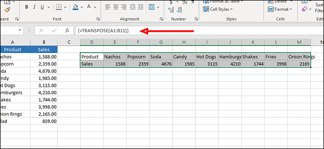
Our data is there now, but the result is a bit messy due to our lack of precision. Let's fix that now. To correct the data, just go back to the formula bar and hit Ctrl + Shift + Enter one more time.

Transposing data with direct references

In our third Excel data transpose method we will use direct references. This method allows us to find and replace a reference with the data that we want to show instead..

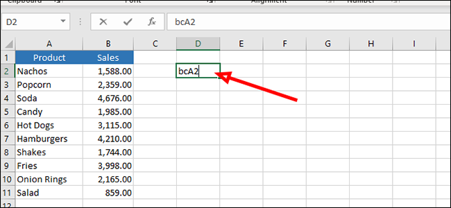
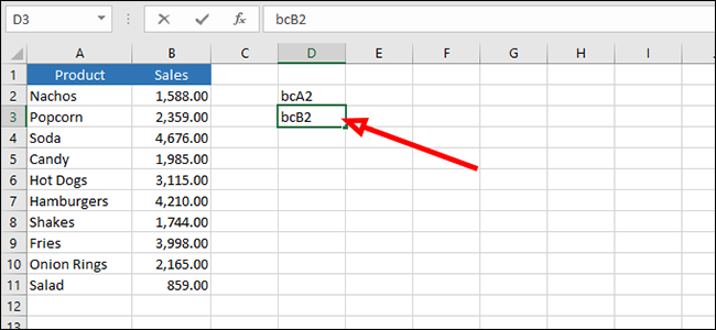
Click on an empty cell and type a reference and then the location of the first cell we want to transpose. I will use my initials. In this circumstance, i will use bcA2.

In the next cell, below the first, write the same prefix and then the cell location to the right of the one we used in the previous step. For our purposes, that would be cell B2, which we will write as bcB2.

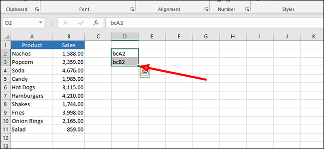
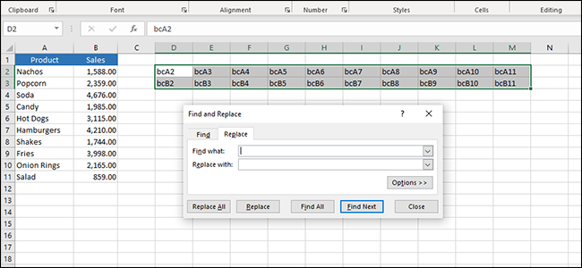
Highlight both cells and drag the highlighted area outward by clicking and dragging the green box at the bottom right of our selection.

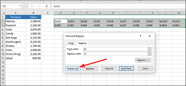
Presione Ctrl + H on your keyboard to open the menu “Search for and replace”.

Enter your selected prefix, “bc” in our case (without quotation marks), in the countryside “Search what”, and then “=” (without quotation marks) in the countryside “Replace with”.

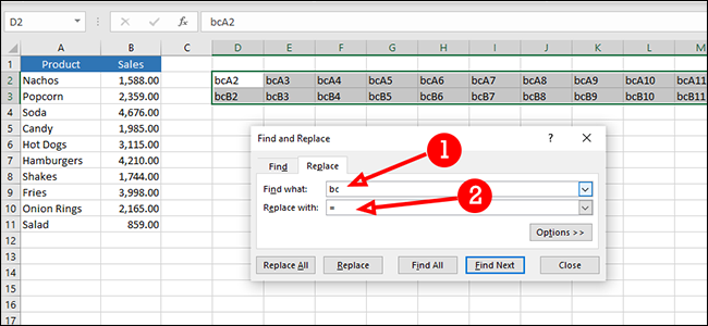
Click the button “Replace all” to transpose your data.

You might be wondering why we didn't add “= A2” to the first empty cell and then drag it to auto-fill the rest.. The reason for this is due to the way Excel interprets this data. Actually, will automatically fill the next cell (B2), but you will run out of data quickly because C3 is empty cell and Excel reads this formula from left to right (because that's the way we drag when transposing our data) instead of top to bottom.