![]()
If you are looking for a unique way to represent your data in Microsoft Excel, consider using icon sets. In a similar way to the color scales, icon sets take a range of values and use visual effects to symbolize those values.
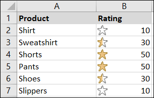
With a conditional formatting rule, can display icons such as traffic lights, stars or arrows depending on the values you enter. As an example, can display an empty star for a value of 10, a star partially filled by 30 and a full star filled by 50.
This feature is great for things like using a rating system, show completed tasks, represent sales or show a change in finances.
Apply a quick conditional formatting icon set
Same way as other conditional formatting rules in Excel, how to highlight higher or lower ranking values, you have some quick options to select. These include basic icon sets that use three, four or five categories with a range of preset values.
Select the cells you want to apply the formatting to by clicking the first cell and dragging the cursor across the rest.
After, open the Home tab and go to the Styles section of the ribbon. Click on “Conditional format” and move the cursor to “Icon sets”. You will see those quick options listed.
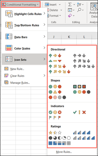
Hovering over the various icon sets, you can preview them on your spreadsheet. This is a nifty way to see which icon set works best for you..
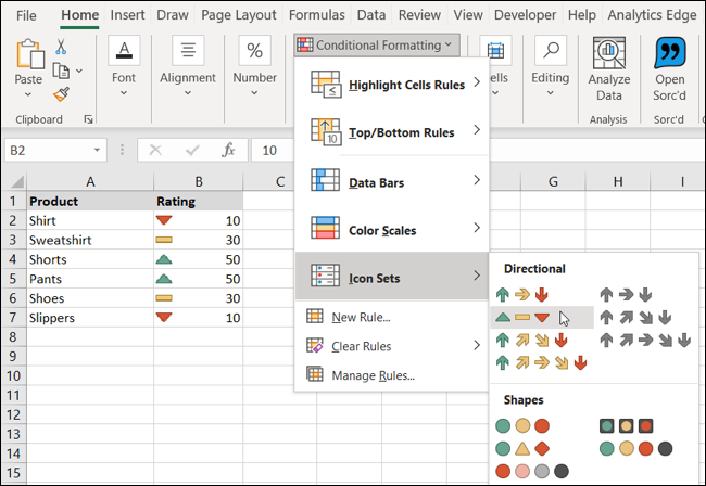
If you find one you want to use, just click on it. This applies the conditional formatting rule to the selected cells with the icon set you chose. As you can see in the screenshot below, we select the stars from our initial example.
Create a custom conditional formatting icon set
As mentioned previously, These Pop-up Menu Icon Set options have presets attached. Because, if you need to adjust the ranges to match your sheet data, you can create a custom conditional formatting rule. And it's easier than you think!!
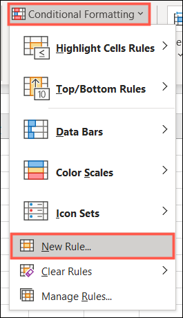
Select the cells where you want to apply the icons, go to the Home tab and choose “New rule” in the Conditional Format drop-down list.
When the New Formatting Rule window opens, select “Format all cells according to their values” at the top.
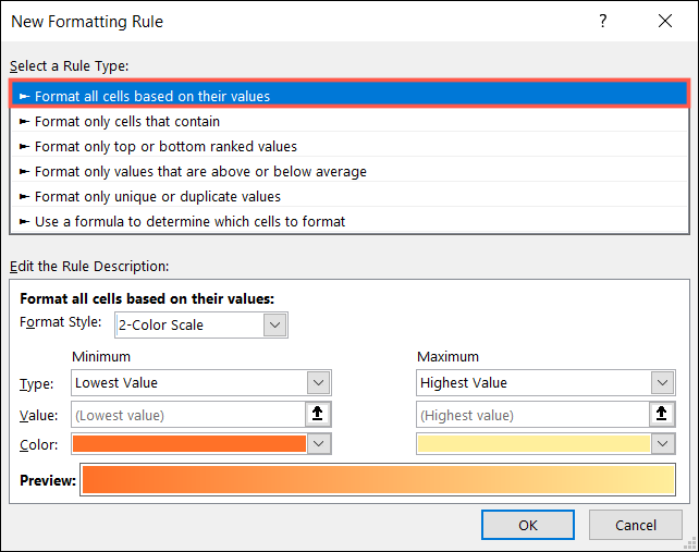
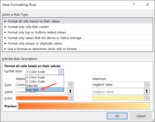
At the bottom of the window, click the Format style drop-down list and select “Icon sets”. After, will customize the rule details.
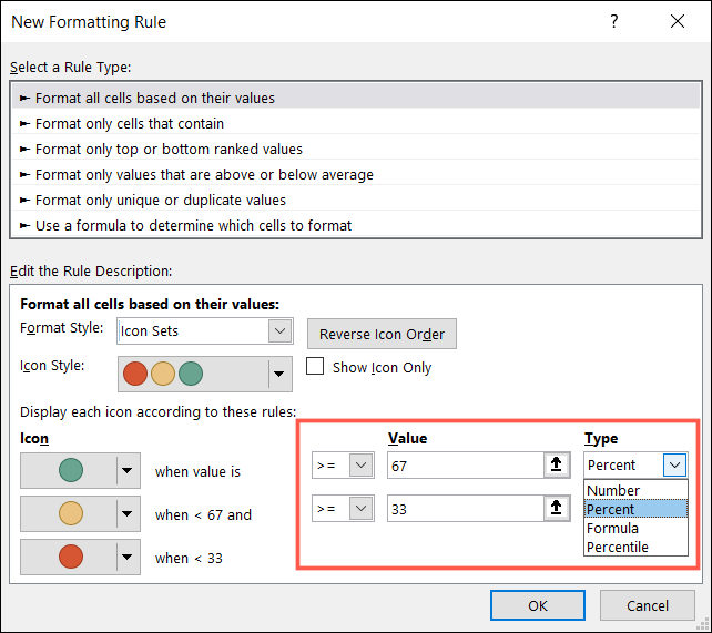
Choose the Icon Style from the next drop-down list. Again, you can select from three, four or five categories. If you prefer the icons in the opposite arrangement, click on “Reverse order of icons”.
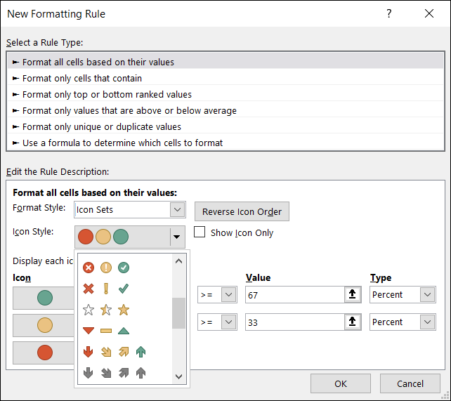
A useful feature of the Icon Sets custom rule is that you are not stuck with the exact set of icons you select. Below the Icon Style drop-down box, you will see boxes for group icons. This enables you to customize the exact icons for your ruler.. Then, and, as an example, you want to use a star, a flag and an arrow instead of three stars, Do it!
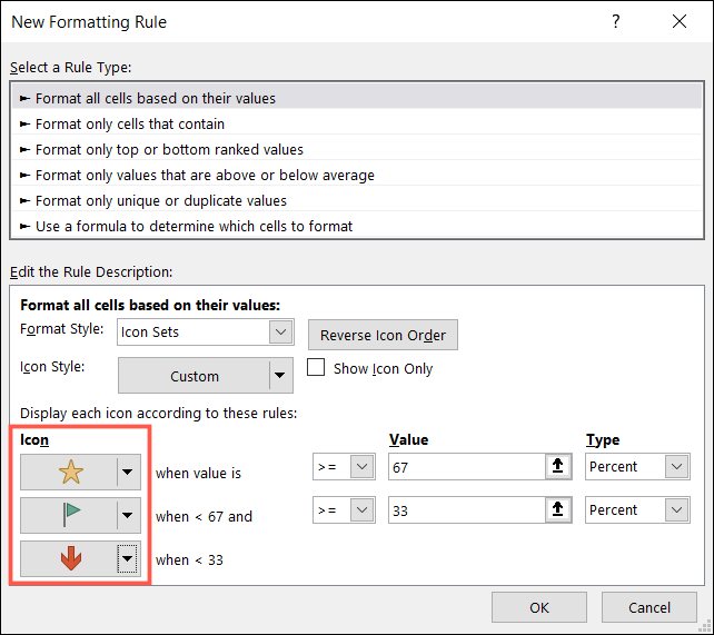
The final part of setting up your rule is entering the values for the range. Choose “Greater than” (>) O “Greater than or equal to” (> =) in the first drop down box. Enter your value in the box below and choose if it is a number, a percentage, a formula or percentile. This gives you great flexibility in setting up your rule..
Now, click on “To accept” to apply your rule.
Another useful feature that is important to note is that it can only display the icon. By default, Excel displays both the icon and the value you enter. But there may be cases where you plan to rely solely on the icon. Then, check the box “Show icon only”.
This is a great example of using icon sets where you only want to display the icon.
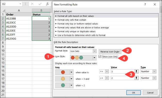
We want to show traffic light icons in green, yellow and red to indicate if our order is new, ongoing or complete. To do it, we will simply enter the numbers one, two or three. As you can see, values are not important in this scenario. They are only used to activate the icon, what do we want to see.
Then, we do the following:
- Select our traffic light icons from three categories.
- Reverse the order (because we want the largest number to be represented by red).
- Enter our values “3” and “2” What “Numbers”.
- Check the box to show only the icon.
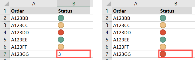
Now, all we will do on our sheet is write “1” for new orders, “2” for those who are in progress and “3” for complete orders. When we press Enter, all we see is our green stoplight indicators, yellow and red.
Hopefully, This tutorial for using icon sets in Microsoft Excel will instruct you to take advantage of this wonderful feature. And to see another way to use conditional formatting, take a look at how to create progress bars in Excel.