How to use the XLOOKUP function in Microsoft Excel

Excel's new XLOOKUP will replace VLOOKUP, providing a powerful replacement to one of the most popular Excel functions. This new feature solves some of the limitations of VLOOKUP and has additional functionality. This is what you need to know.

What is XLOOKUP?

The new XLOOKUP feature has fixes for some of VLOOKUP's biggest limitations. At the same time, also replaces HLOOKUP. As an example, XLOOKUP can look to your left, by default it is an exact match and enables you to specify a range of cells instead of a column number. VLOOKUP is not so easy to use or so versatile. We will show you how it all works.

For the moment, XLOOKUP is only enabled for Insiders program users. Anyone can join the Insiders program to access the latest Excel functions as soon as they are available. Microsoft will soon start rolling it out for all Office users 365.

How to use the XLOOKUP function

Let's dive right into an example of XLOOKUP in action. Take the example data below. We want to return the department of column F for each ID in column A.

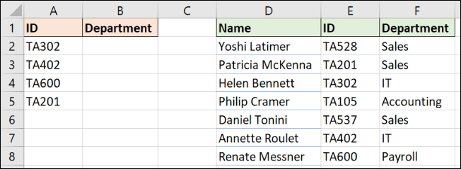
This is a classic exact match search example. The XLOOKUP function needs only three pieces of information.

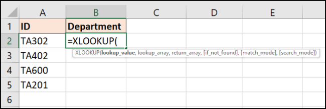
The next image shows XLOOKUP with six arguments, but only the first three are required for an exact match. So let's focus on them:

• Search value: What are you looking for.
• Lookup_array: Where to look.
• Return_array: the range containing the value to return.

The following formula will work for this example: =XLOOKUP(A2,$E$2:$E$8,$F$2:$F$8)

Let's now explore a couple of advantages that XLOOKUP has over VLOOKUP here.

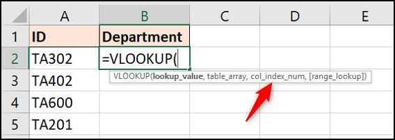
No more column index number

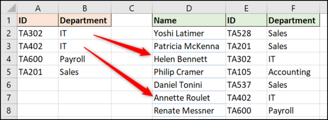
The infamous third argument to VLOOKUP was to specify the column number of information to return from a table array. This is no longer an obstacle as XLOOKUP allows you to choose the range from which to return. (column F in this example).

And don't forget, XLOOKUP can see the data left from the selected cell, unlike VLOOKUP. More on this below.

At the same time, no longer have the problem of a broken formula when new columns are inserted. If that happened in your spreadsheet, the return range would be adjusted automatically.

Exact match is the default

It was always confusing when learning VLOOKUP why you had to specify an exact match.

Fortunately, XLOOKUP defaults to an exact match, the much more common reason to use a search formula). This reduces the need to answer that fifth argument and ensures fewer errors from users new to the formula..

Then, In summary, XLOOKUP asks fewer questions than VLOOKUP, it is easier to use and is also more durable.

XLOOKUP can look to the left

Being able to choose a search range makes XLOOKUP more versatile than VLOOKUP. With XLOOKUP, the order of the table columns does not matter.

VLOOKUP was restricted by searching in the leftmost column of a table and then returning from a specified number of columns to the right.

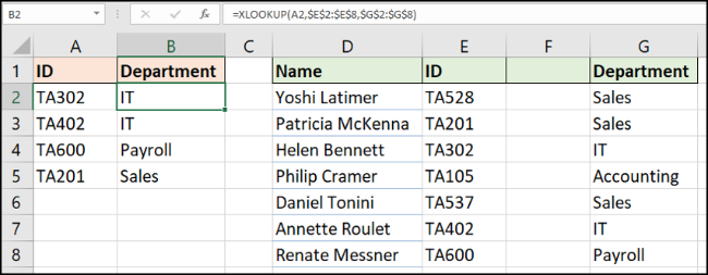
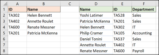
In the following example, we need to look for an id (column E) and return the person's name (column D).

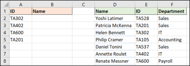
The following formula can achieve this: =XLOOKUP(A2,$E$2:$E$8,$D$2:$D$8)

What to do if not found

Users of search functions are very familiar with the error message # N / Say hello to them when their VLOOKUP or MATCH function can't find what they need. And there is often a logical reason for this.

Because, users quickly research how to hide this error because it is neither correct nor useful. AND, in any case, there are alternatives to do it.

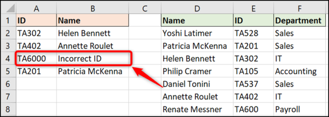
XLOOKUP comes with its own argument “if not found” built-in to handle such errors. Let's see it in action with the example above, but with a misspelled ID.

The next formula will display the text “ID incorrecta” instead of the error message: =XLOOKUP(A2,$E$2:$E$8,$D$2:$D$8,"Incorrect ID")

Using XLOOKUP for a range search

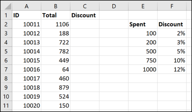
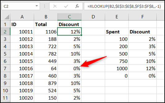
Even though it is not as common as the exact match, a very effective use of a search formula is to search for a value in ranges. Take the following example. We want to return the discount based on the amount spent.

This time we are not looking for a specific value. We need to know where the values ​​of column B lie within the ranges of column E. That will determine the discount obtained.

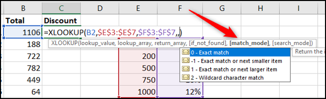
XLOOKUP has an optional fifth argument (remember, defaults to the exact match) called matching mode.

You can see that XLOOKUP has greater capabilities with fuzzy matches than VLOOKUP.

There is an option to find the closest match less than (-1) or closer greater than (1) the value sought. Also there is an option to use wildcard characters (2) What? o la *. This setting is not enabled by default as it was with VLOOKUP.

The formula in this example returns the closest less than the searched value if no exact match is found: =XLOOKUP(B2,$E$3:$E$7,$F$3:$F$7,,-1)

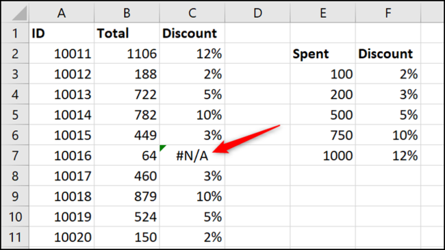
Despite this, there is an error in cell C7 where the error is returned # N / A (the 'if not found' argument was not used). This should have returned a 0% off because you spend 64 does not meet the criteria for any discount.

Another advantage of the SEARCH X function is that you don't need the search range to be in ascending order like VLOOKUP does..

Enter a new row at the bottom of the lookup table and then open the formula. Expand the range used by clicking and dragging the corners.

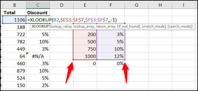
The formula immediately fixes the error. It is not an obstacle to have the “0” at the bottom of the range.

Personally, would still sort the table by the lookup column. Have a “0” at the bottom I would go crazy. But the fact that the formula was not broken is brilliant.

XLOOKUP also overrides the HLOOKUP function

As mentioned, the XLOOKUP function is also here to replace HLOOKUP. One function to replace two. Excellent!

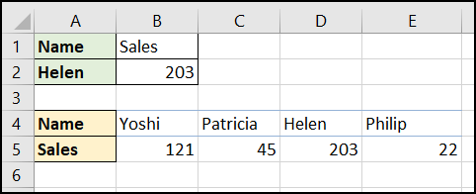
HLOOKUP function is horizontal search, used to search across rows.

He is not as well known as his brother VLOOKUP, but it is useful for examples like the one shown below, where the headings are in column A and the data is in the rows 4 and 5.

XLOOKUP can look in both directions: columns down and further along rows. We no longer need two different functions.

In this example, the formula is used to return the sales value related to the name in cell A2. Search along the line 4 to find the name and return the value of the row 5: =XLOOKUP(A2,B4:E4,B5:E5)

XLOOKUP can look from the bottom up

In general, you must search a list to find the first (often unique) appearance of a value. XLOOKUP has a sixth argument called search mode. This allows us to change the search to start at the bottom and search a list to find the last occurrence of a value.

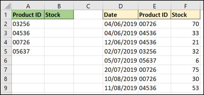
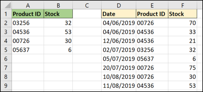
In the following example, we would like to find the stock level of each product in column A.

The lookup table is sorted by date and there are multiple stock checks per product. We want to return the stock level from the last time it was checked (last occurrence of the product ID).

The sixth argument of the SEARCH X function offers four options. We are interested in using the option “Search from last to first”.

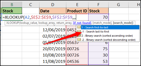
The full formula is shown here: =XLOOKUP(A2,$E$2:$E$9,$F$2:$F$9,,,-1)

In this formula, the fourth and fifth arguments were ignored. It is optional and we wanted the default value of an exact match.

Rounding

The XLOOKUP function is the eagerly awaited successor to the VLOOKUP and HLOOKUP functions.

In this post several examples were used to demonstrate the benefits of XLOOKUP. One of them is that XLOOKUP can be used on sheets, workbooks and also with tables. The examples were kept simple in the post to help our understanding.

Because dynamic arrays that are entered in Excel early, it can also return a range of values. Definitely, this is something that is important to highlight explore further.

VLOOKUP days are numbered. XLOOKUP is here and will soon be the de facto search formula.