You can add a trend line to a chart in Excel to show the general pattern of data over time. You can also expand trend lines to forecast future data. Excel makes all of this easy.
A trend line (or line of best fit) is a straight or curved line that displays the general direction of the values. In general, are used to show a trend over time.
In this post, we will cover how to add different trend lines, format and extend them for future data.
Add a trend line
You can add a trend line to an Excel chart in just a few clicks. Let's add a trend line to a line chart.
Select the chart, Click the button “Chart items” and then click the checkbox “Trend line”.
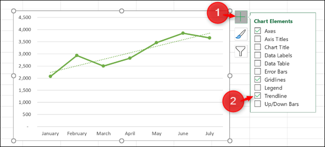
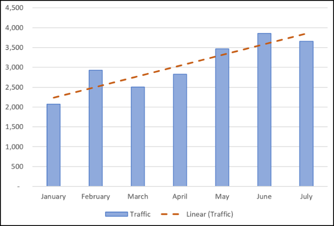
This adds the default linear trend line to the chart.
There are different trend lines available, so it is a good idea to select the one that best suits your data pattern.
and then click the checkbox “Trend line” and then click the checkbox other trend lines, including moving average or exponential.
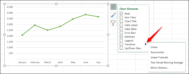
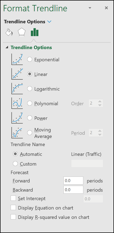
Some of the key trend line types include:
- Lineal: A straight line that is used to show a constant rate of increase or decrease in values.
- Exponential: This trend line visualizes an increase or decrease in values at an increasing rate. The line is more curved than a linear trend line.
- Logarithmic: This type is best used when data is rapidly increasing or decreasing and then leveling out.
- Moving average: To smooth fluctuations in your data and show a trend more clearly, use this type of trend line. Use a specific number of data points (two is the default), averages them and then uses this value as a point on the trend line.
To see the full complement of alternatives, click on “More options”.
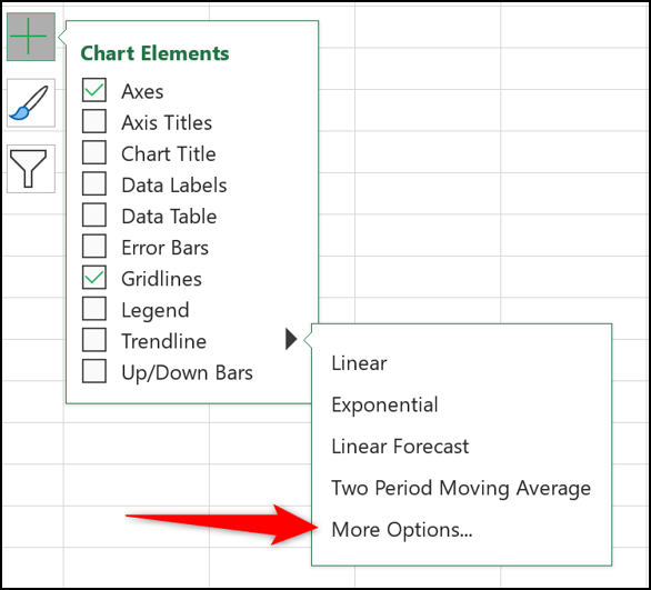
The Format Trendline panel opens and presents all the trendline types and other options. We will explore more of these later in this post..
Choose the trend line you want to use from the list and it will be added to your chart.
Add trend lines to multiple data series
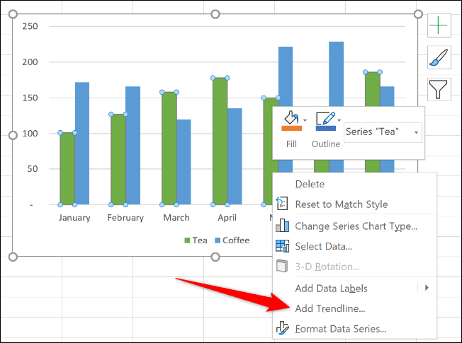
In the first example, the line chart had only one data series, but the following column chart has two.
If you want to apply a trend line to only one of the data series, right click on the desired item. Next, select “Add trend line” on the menu.
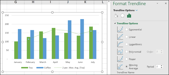
The Format Trendline panel opens so you can choose the trendline you want.
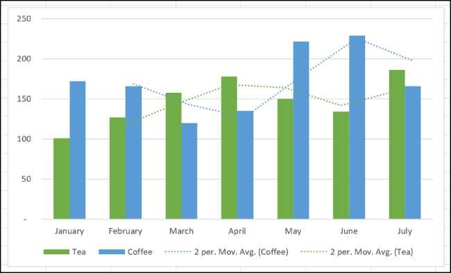
In this example, a moving average trend line has been added to the Tea data series charts.
This is probably your directory “Chart items” and then click the checkbox, Excel asks which data series you want to add the trend line to.
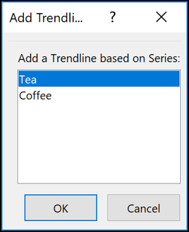
You can add a trend line to multiple data series.
In the next picture, a trend line has been added to the tea and coffee data series.
Additionally you can add different trend lines to the same data series.
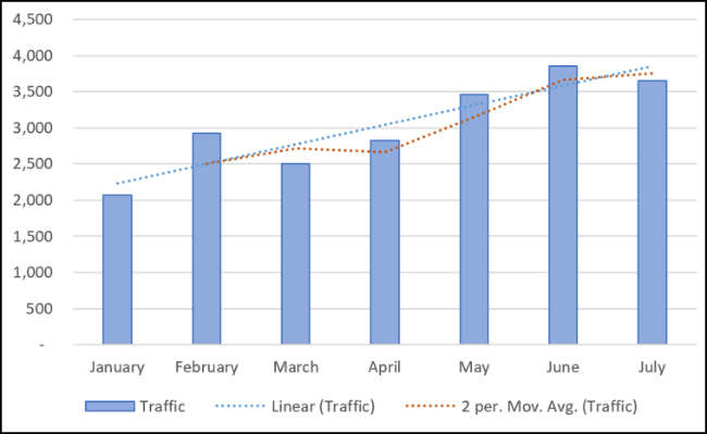
In this example, linear trend lines and moving average have been incorporated into the chart.
Format your trend lines
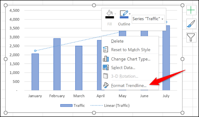
Trend lines are added as a dashed line and match the color of the data series to which they are mapped. You may want to format the trend line differently, especially if you have multiple trend lines on one chart.
and then click the checkbox “Format trend line”.
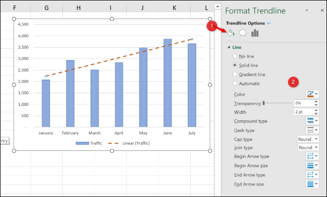
Click the Fill & Line category, and later you can choose a line color, width, different stroke type and more for your trend line.
In the following example, i changed the color to orange, so it is different from the column color. Also I increased the width to 2 points and changed the dash type.
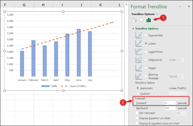
Expand a trend line to forecast future values
A very cool feature of trend lines in Excel is the option to extend them in the future. This gives us an idea of what future values could be based on the current trend of the data..
In the Format Trendline panel, and then click the checkbox “Ahead” under “Forecast”.
Show R-squared value
The R-squared value is a number that indicates how well your trend line matches your data.. The closer to 1 let the value of R squared, the better the trend line fit.
In the Format Trendline panel, excel template “Trend line options” and then click the checkbox “Show R-squared value on graph”.
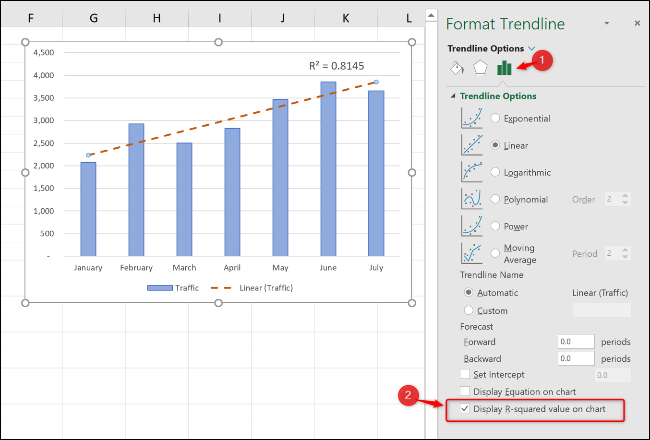
A value of 0,81. This is a reasonable accommodation, since a value greater than 0,75 generally considered decent; the closer to 1, better.
If the value of R squared is low, you can test other types of trend lines to see if they fit your data better.